Repository navigation
Low-mode TAE examples: initial width sigma 0.1 and hole a1 = 0.01 (as the ITPA examples) - #915
Merged
Merged
Conversation


….01 (flag --a1)

The m = 1, 2 velocity harmonics of the initial condition have the radial width 0.1 of the
ITPA TAE examples (was 0.15), and the hole around the magnetic axis has the radius 0.01 by
default (was 0.1; new flag --a1 as in the ITPA examples). ShearAlfven (Hdiv, 4 ranks):
omega = 0.0632, expected 0.0672 (was 0.0631 with sigma 0.15, a1 0.1).

Co-Authored-By: Claude Opus 5.5 <noreply@anthropic.com>
…DKCC results of the earlier defaults

Co-Authored-By: Claude Opus 5.5 <noreply@anthropic.com>

spossann
marked this pull request as ready for review
November 10, 2026 15:38
spossann
added a commit
that referenced
this pull request
Nov 10, 2026

…; videos in lowmode_tae (#913) ## Summary Generic frames for videos of FEEC fields in pproc scripts, and videos of the radial velocity in the `ShearAlfven/lowmode_tae` example. New module `struphy.post_processing.frames`: - `write_slice_frames(out, name, folder, component=..., basis="norm", plane="rz", ...)`: the field in a physical plane (`xy`, `xz`, `yz`, `rz`, as in `slices.py`), with matplotlib. - `write_3d_frames(out, name, folder, component=..., view="cut" | "domain", ...)`: 3D with a cutaway, with PyVista. The view and the cut are fixed over the video. The cut is placed at the largest value over all frames, moved between two planes of grid points. The title and colour bar are added with matplotlib around the cropped render. - The boundary of the domain is translucent (`opacity=0.35`), while the faces of the cut stay opaque. - An opaque surface eta1 = const goes through the largest absolute value (`surface="peak"`), e.g. the flux surface of the TAE. Together they show the toroidal mode structure. - Both settings apply to the `"cut"` and the `"domain"` view. - Both: - One PNG per saved time step: `frame_0000.png`, … plus `frames.txt` (step and time). - At most `max_frames=500`, evenly spaced, including the first and last step. - One colour scale over the whole video by default (`clim="frame"` gives one per frame, or pass `(vmin, vmax)`). - The same even pixel size in all frames, so ffmpeg can use them directly. - What is shown: a scalar field, one component of a vector field in any basis (`"norm"`, `"1"`, `"2"`, `"v"`, `"physical"`), or the magnitude of a vector field. - Values come from the saved spline coefficients, so no `pproc` or VTK files are needed. - On polar domains, the singular values on the axis are replaced by those of the next ring. - Frames are written on rank 0 only. - `frames_to_video(folder, fps=25)`: makes an MP4 with ffmpeg (optional; you can also make the video yourself from the PNGs). - `write_videos(out, name, folder, component=0, prefix="u_r")`: all standard videos of a field in one call. That is `<prefix>_rz` for tori and cylinders, or every plane of the domain (e.g. `u_r_xy`, `u_r_xz`, `u_r_yz` for a slab), plus `<prefix>_3d_cut` and `<prefix>_3d`. - Titles show the time as `t = <t>/<end time>`, e.g. `t = 124/600`, for orientation. - **Any domain**: - `slices.physical_planes` treats Colella and Orthogonal like Cuboid; their mid-planes are flat, and a test checks it. - Other domains no longer raise a `NotImplementedError`; the new `logical_mid_planes` gives: - other tori (Tokamak, GVEC, DESC): the poloidal plane `rz` at eta3 = 0.5, in R and z; - everything else: the logical mid-surfaces `eta3`, `eta2`, and `eta1` only with `all_planes`. - Domains covering only part of the poloidal angle get the 3D views only, with a warning. - Tested with short slab and Colella runs. - The default 3D resolution adapts to at most about 1e6 points: 4 points per cell for the low-mode tori, 2 for the ITPA tori with `tor_period=6`. - Sharp edges (slabs, cut faces) are shaded as edges. `plot_3d.py`: - The rendering is split into helpers used by both `plot_field_3d` and the frames: `cut_center`, `peak_azimuth`, `merge_seams`, `new_plotter`, `add_field_mesh`, `set_camera`, `crop_box`. - New `off_grid_azimuth`. A cut exactly through a plane of grid points left degenerate cells, drawn as dark specks on the cut face. The existing standard 3D plots get this fix as well. All TAE examples write the videos: - `lowmode_tae` and `itpa_tae_benchmark` of ShearAlfven, LinearMHD and LinearMHDDriftkineticCC (both the B0 and the Bmax case); - `lowmode_tae` of PerturbativeMHDWithQDriftkineticCC, VariationalLinearMHD and VariationalPerturbativeLinearMHD (`with_q`). Each one writes three videos of the radial velocity u\_r (component 0 in the normalized basis) into `<path_out>/results/frames/`: - `u_r_rz`: the poloidal plane. - `u_r_3d_cut`: 3D, camera on the cut face. - `u_r_3d`: 3D, the whole torus. - New flags `--no-frames` and `--max-frames`. The usage guide (`postprocess-simulation` skill) has a new section "Videos of fields". ## Figures Full ShearAlfven `lowmode_tae` run: - Default `--b-space Hdiv`, 16×16×8 grid, 1200 steps, 4 ranks, about 12 min. - New low-mode parameters of PR #915: initial width sigma = 0.1, hole a1 = 0.01. - The measured TAE frequency is 0.0632, expected 0.0672 (within the 10% tolerance). - The 301 frames per video take about 3–5 min each. GIFs: every 2nd frame, 480 px wide (the PNG frames are at full resolution). | poloidal plane `u_r_rz` | 3D, whole torus `u_r_3d` | 3D, cut face `u_r_3d_cut` | |---|---|---| | 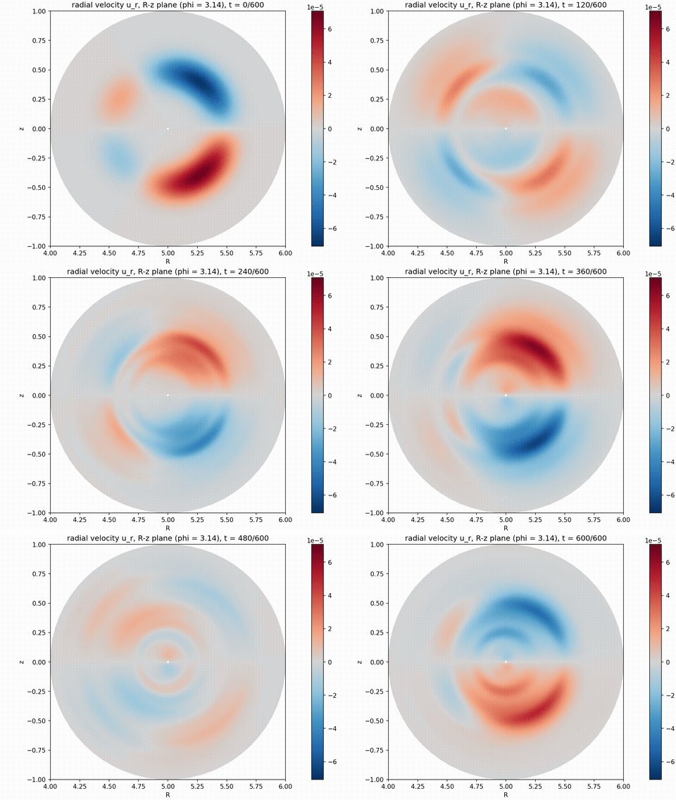 | 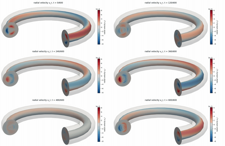 | 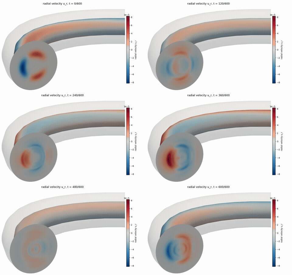 | Single full-resolution frames at t = 300: 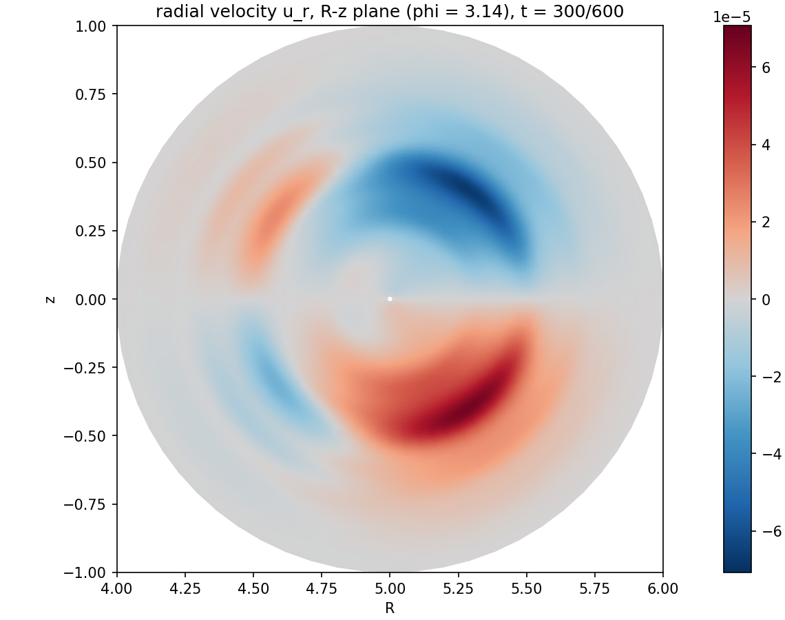 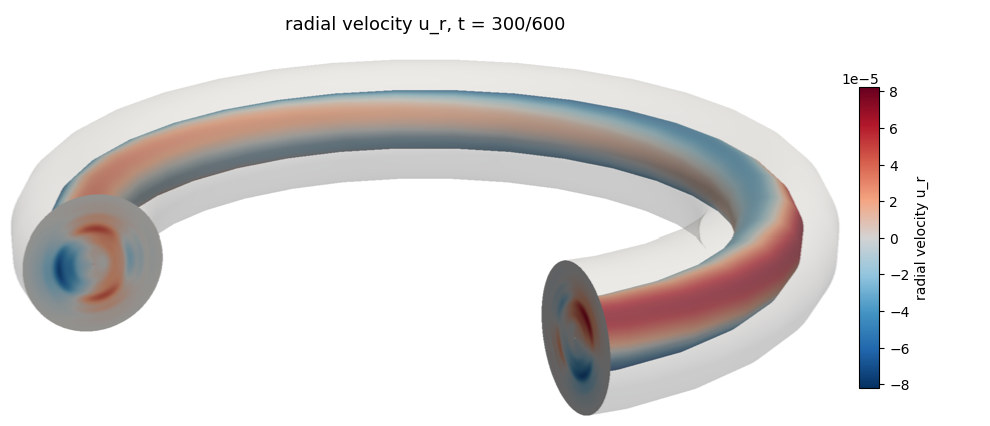 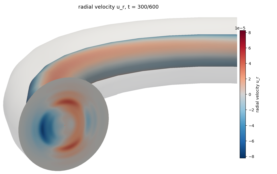 (The figures are on the branch `pr-figures/pproc-frames`, which is not to be merged and can be deleted after the review.) ## Tests - All 10 TAE examples pass with `--test-run` plus pproc on 2 ranks, 3 videos each, 30–75 s per example. - `test_frames.py`, `test_slices.py` and `test_plot_3d.py`: 54 passed serially; the frames tests also pass on 2 MPI ranks. - New since the first version: slab and Colella videos, the flat Colella/Orthogonal planes, and the R-z fallback for tori. - A second review agent checked commit a380a32; its findings are fixed in a4695e2: - other tori in R-z; - partial poloidal angles; - the `SKILL.md` import; - cube-root round-off in the adaptive resolution; - docstrings; - frame-count prints on rank 0 only. - `post_processing/tests/test_frames.py`: - Short Maxwell runs on a HollowTorus and on an IGAPolarTorus with polar splines (axis). - Both writers and both views, the `physical` basis, `clim` modes, validation and `frames_to_video`. - Unit tests of `off_grid_azimuth`, the axis fix and the colour limits. - Passes serially (with `test_plot_3d.py`: 14 passed) and on 2 MPI ranks. - The tests folder is already in a shard. - ruff check and format are clean. - A separate review agent checked the first commit; its findings are fixed in the second one: - axis inf/NaN on polar domains; - frame times in the time units of the `Output`; - spline snapshots of the frames evicted from the `Output` cache; - the second cut face also off-grid; - validation of `max_frames` and `clim`. 🤖 Generated with [Claude Code](https://claude.com/claude-code) --------- Co-authored-by: Claude Opus 5.5 <noreply@anthropic.com>
This file contains hidden or bidirectional Unicode text that may be interpreted or compiled differently than what appears below. To review, open the file in an editor that reveals hidden Unicode characters.
Learn more about bidirectional Unicode characters
Sign up for free
to join this conversation on GitHub.
Already have an account?
Sign in to comment







Add this suggestion to a batch that can be applied as a single commit.This suggestion is invalid because no changes were made to the code.Suggestions cannot be applied while the pull request is closed.Suggestions cannot be applied while viewing a subset of changes.Only one suggestion per line can be applied in a batch.Add this suggestion to a batch that can be applied as a single commit.Applying suggestions on deleted lines is not supported.You must change the existing code in this line in order to create a valid suggestion.Outdated suggestions cannot be applied.This suggestion has been applied or marked resolved.Suggestions cannot be applied from pending reviews.Suggestions cannot be applied on multi-line comments.Suggestions cannot be applied while the pull request is queued to merge.Suggestion cannot be applied right now. Please check back later.
Summary
Low-mode TAE examples: new defaults for the initial condition and the domain, to match the ITPA TAE examples.
--a1, as in the ITPA examples.Affected
lowmode_taeexamples:with_q.The descriptions are updated accordingly.
Verification
Full runs with the new defaults, 4 ranks:
--test-runplus pproc on 2 ranks. This was checked on the base of Video frames of FEEC fields (2D planes, 3D cutaway) for pproc scripts; videos in lowmode_tae #913, where VariationalLinearMHD was stillVariationalPerturbativeLinearMHD/with_p; CI runs them on devel.The video PR #913 shows its figures from the ShearAlfven run with these defaults.
🤖 Generated with Claude Code