Source Code of Continuous Deep Q-Learning with Simulator for Stabilization of Uncertain Discrete-Time Systems (Sim-CDQL)

Pre-train DNN's paramete vectors are in weight_DNN.

https://arxiv.org/abs/2101.05640

The example of a discrete-time system is a pendulum dynamics computed by Euler-method with stepsize 2**(-4). We describe the dynamics in Pendulum.pdf (https://github.com/pondbooks/CDQL_with_Sim/blob/main/Pendulum.pdf). The range of an angle is [-np.pi, np.pi].

Normalize an angle

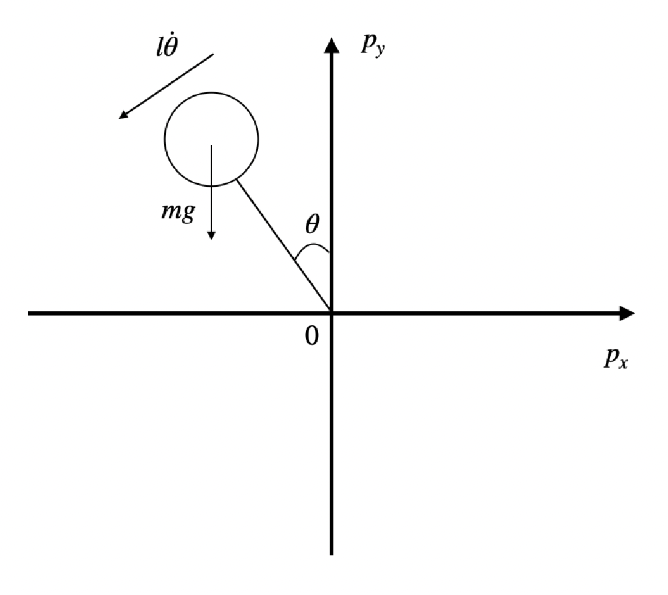
We use the np.arctan2(y, x) function (https://numpy.org/doc/stable/reference/generated/numpy.arctan2.html) for normalization of an angle parameter. The range of the angle parameter is [-np.pi, np.pi]. At first, the angle_normalize obtains an angle parameter theta. Secondly, the function computes the y-coordinate y and x-coordinate x by np.sin(theta) and np.cos(theta), respectively. Finally, the function computes the normalized angle by np.arctan2(y,x).

def angle_normalize(theta):
  x_plot = np.cos(theta)
  y_plot = np.sin(theta)
  angle = np.arctan2(y_plot,x_plot)
  return angle

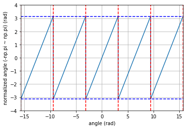
This Fig. shows the angle normalize function in the range [-5*np.pi, 5*np.pi]. The red lines show the angles = -5*np.pi, -3*np.pi, -np.pi, np.pi, 3*np.pi, 5*np.pi. The blue lines show the normalized angles = -3*np.pi, 3*np.pi.

warning (2022/4/10)

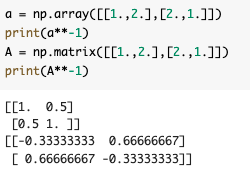
In this source code, we use A**(-1) for computing an inverse matrix. However, in this case, we must define the matrix as np.matrix. So, we should change A**(-1) to np.linalg.inv(). In this example, fortunately, we consider the 1-dim problem. We can obtain the same result.

PC

CPU: Intel Core i7-10700 (1200/2.9/16M/C8/T16)

Memory: Samsung M378A2K43CB1-CTD (DDR4 PC4-21300) 16GB×2

Motherboard: ASUS PRIME H470-PLUS (H470 1200 DDR4 ATX)I

GPU: NVIDIA(R) GeForce RTX 2070 SUPER

OS: windows10

Python: 3.6.10

Pytorch: 1.5.1

matplotlib: 3.3.0

numpy: 1.18.5