RPE Cells
- Needed packages
- Needed data
- Section 1: Studying Dividing Daughter Cells
- Section 2: Plotting the lineage tree
- Section 3: Generation plot for all the data
- Section 4: Heterogeneity between daughter cells
- Section 5: Changes across cell cycle phases
require(tidyverse)
require(igraph)
require(ggplot2)
require(vioplot)All the needed data are available here
The notebook consists of five sections
First we create a path string that stores the location of the files:
path <- "../Data/RPE tracking data/" # You may need to change thisNow we can properly read the files.
df <- read.csv(file.path(path, "PIP-FUCCI Dividing Daughter Cells.csv"))
head(df)
## ExperimentName TiffFileName CellName isDivided isDaughter nImages Distance Displacement TrajectoryTime Directionality
## 1 PIP-FUCCI PIP-FUCCI.tif C3.1 TRUE TRUE 123 178.1 27.7 1220 0.156
## 2 PIP-FUCCI PIP-FUCCI.tif C3.1.1 TRUE TRUE 113 127.2 40.5 1120 0.319
## 3 PIP-FUCCI PIP-FUCCI.tif C3.1.2 TRUE TRUE 126 126.7 32.0 1250 0.253
## 4 PIP-FUCCI PIP-FUCCI.tif C3.2 TRUE TRUE 133 181.2 9.8 1320 0.054
## 5 PIP-FUCCI PIP-FUCCI.tif C3.2.2 TRUE TRUE 149 224.2 16.1 1480 0.072
## 6 PIP-FUCCI PIP-FUCCI.tif C4.1 TRUE TRUE 103 237.3 20.2 1020 0.085
## AverageSpeed
## 1 0.146
## 2 0.114
## 3 0.101
## 4 0.137
## 5 0.151
## 6 0.233
dim(df)## [1] 48 11
TrajectoryTime <- df[, 9]/60
sd(TrajectoryTime)
## [1] 4.761354
summary(TrajectoryTime)## Min. 1st Qu. Median Mean 3rd Qu. Max.
## 12.67 18.92 20.67 21.52 23.21 41.33
x <- TrajectoryTime
hx5 <- TrajectoryTime
dens <- density(hx5, cut=10)
n <- length(dens$y)
dx <- mean(diff(dens$x))                  # Typical spacing in x
y.unit <- sum(dens$y) * dx                # Check: this should integrate to 1
dx <- dx  /  y.unit                       # Make a minor adjustment
x.mean <- sum(dens$y * dens$x) * dx
y.mean <- dens$y[length(dens$x[dens$x < x.mean])]
x.mode <- dens$x[i.mode <- which.max(dens$y)]
y.mode <- dens$y[i.mode]
y.cs <- cumsum(dens$y)
x.med <- dens$x[i.med <- length(y.cs[2 * y.cs <= y.cs[n]])]
y.med <- dens$y[i.med]plot(
dens, type="l", col="black", lwd=0.1, xlim=c(0, 50), cex=1.5, cex.lab=1.3,
cex.axis=1.3, xlab="The doubling time of hTERT-immortalized RPE cells (h)"
)
polygon(dens, col="black")
temp <- mapply(
function(x, y, c) lines(c(x, x), c(0, y), lwd=2, col=c, las=1),
c(x.mean, x.med, x.mode),
c(y.mean, y.med, y.mode),
c("orange", "Green", "Red")
)
legend(
28.5, 0.115, c("Doubling Time Density", "Mode", "Median", "Mean"),
col=c("black", "Red", "green", "orange"), text.col="black", lty=1, lwd=2,
cex=1, merge=TRUE
)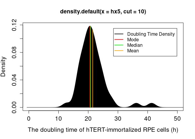
cat("The mode doubling time is ",x.mode,"\n" )## The mode doubling time is 20.56724
Directionality <- df[, 10]
Group <- c(rep(1, length(Directionality)))
Da <- data.frame(Directionality, Group)

#  Add mean and standard deviation within violin plot
data_summary <- function(x) {
    m <- mean(x)
    ymin <- m - sd(x)
    ymax <- m + sd(x)
    return(c(y=m, ymin=ymin, ymax=ymax))
}

p <- ggplot(Da, aes(x=Group, y=Directionality)) +
    geom_violin(trim=FALSE, fill="lightgreen") +
    geom_point(size=2.5, color="black")
p + stat_summary(fun.data=data_summary, geom="pointrange", color="red", size=1)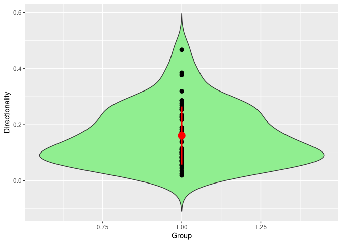
summary(Directionality)## Min. 1st Qu. Median Mean 3rd Qu. Max.
## 0.01900 0.08325 0.14550 0.16094 0.22950 0.46700
sd(Directionality)## [1] 0.1033571
Average_Speed <- df[, 11] * 60
Group <- c(rep(1, length(Average_Speed)))
Da <- data.frame(Average_Speed, Group)
data_summary <- function(x) {
    m <- mean(x)
    ymin <- m - sd(x)
    ymax <- m + sd(x)
    return(c(y=m, ymin=ymin, ymax=ymax))
}
p <- ggplot(Da, aes(x=Group, y=Average_Speed)) +
    geom_violin(trim=FALSE, fill="yellow") +
    geom_point(size=2.5, color="black")
p + stat_summary(fun.data=data_summary, geom="pointrange", color="red", size=1)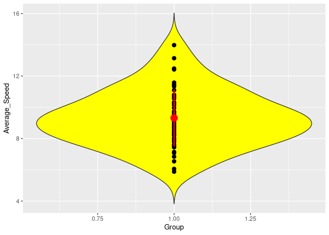
summary(Average_Speed)## Min. 1st Qu. Median Mean 3rd Qu. Max.
## 5.880 8.175 9.180 9.316 10.380 13.980
sd(Average_Speed)## [1] 1.81575
DT <- df[, 9] / 60    # doubling time
f <- df[, 7]          # Total Distance
ff <- as.numeric(gsub(", ", ".", f))
plot(DT,f,xlab="Doubling time (h)",ylab="Total Distance (um)",pch=16,las=0,cex=1.5,cex.lab=1.3, cex.axis=1.3,xlim=c(0,45),ylim=c(0,500))
c <- cor.test(~ DT+ ff, method="pearson", exact=FALSE)
c
##
## Pearson's product-moment correlation
##
## data: DT and ff
## t = 8.953, df = 46, p-value = 1.214e-11
## alternative hypothesis: true correlation is not equal to 0
## 95 percent confidence interval:
## 0.6631669 0.8815754
## sample estimates:
## cor
## 0.7971043
reg <- lm(ff ~ DT)
cc <- unlist(c[4])
ccPV <- round(cc, digits=2)
abline(reg, untf=TRUE, col="red", lwd=2)
text(4, 500, "r= 0.8",cex = 1.5)
text(5.7, 460, "P< 0.001",cex = 1.5)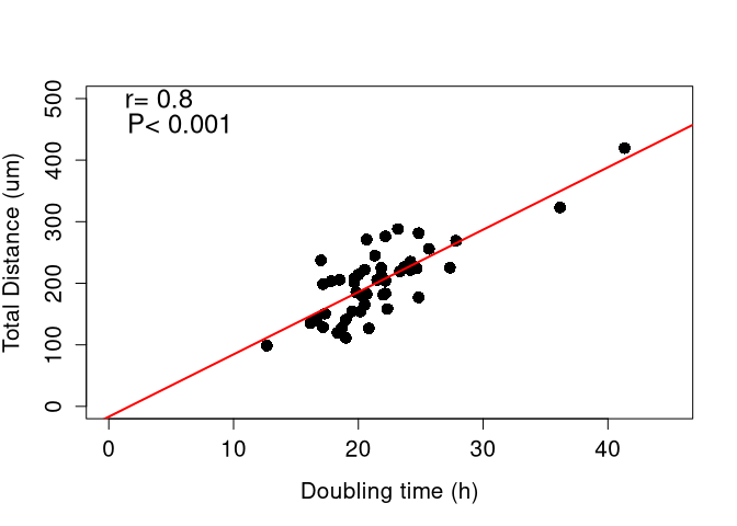
DT <- df[, 9] / 60    # doubling time
f <- df[, 10]         # Directionality
plot(
    DT, f, xlab="Doubling time (h)", ylab="Directionality", pch=16, las=1,
    ylim=c(0, .65)
)
c <- cor.test( ~ DT + f, method="pearson", exact=FALSE)
c
##
## Pearson's product-moment correlation
##
## data: DT and f
## t = -1.9383, df = 46, p-value = 0.05874
## alternative hypothesis: true correlation is not equal to 0
## 95 percent confidence interval:
## -0.51843970 0.01014446
## sample estimates:
## cor
## -0.2747823
reg <- lm(f ~ DT)
cc <- unlist(c[4])
ccPV <- round(cc, digits=2)
abline(reg, untf=TRUE, col="red", lwd=2)
text(19, 0.65, "r= -0.27",cex = 1)
text(19.4, 0.6, "P= 0.059",cex = 1)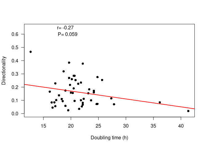
DT <- df[, 9] / 60    # doubling time
f <- df[, 11] * 60    # Average Speed
plot(DT,f,xlab="Doubling time (h)",ylab="Average Speed (um/h)",pch=16,las=1,ylim=c(0,20))
c <- cor.test( ~ DT+ f, method="pearson", exact=FALSE)
c
##
## Pearson's product-moment correlation
##
## data: DT and f
## t = 0.57788, df = 46, p-value = 0.5662
## alternative hypothesis: true correlation is not equal to 0
## 95 percent confidence interval:
## -0.2041630 0.3603391
## sample estimates:
## cor
## 0.08489657
reg <- lm(f ~ DT)
cc <- unlist(c[4])
ccPV <- round(cc, digits=2)
abline(reg, untf=TRUE, col="red", lwd=2)
text(15, 20, "r= 0.08",cex = 1)
text(15.25, 19, "P= 0.57",cex = 1)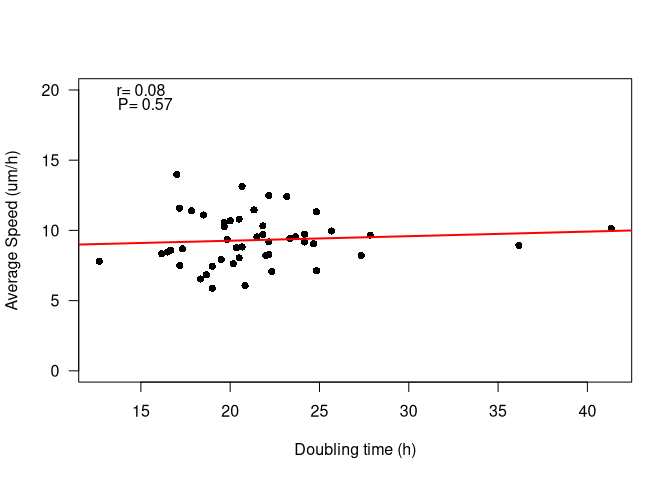
df <- read.csv(file.path(path, "PIP-FUCCI All Cells_Results.csv"))
head(df)
## ExperimentName TiffFileName CellName isDivided isDaughter nImages Distance Displacement TrajectoryTime Directionality
## 1 PIP-FUCCI PIP-FUCCI.tif C1 TRUE FALSE 182 202.9 27.6 1810 0.136
## 2 PIP-FUCCI PIP-FUCCI.tif C1.1 FALSE TRUE 55 82.2 7.4 540 0.089
## 3 PIP-FUCCI PIP-FUCCI.tif C1.2 FALSE TRUE 45 74.2 7.8 440 0.106
## 4 PIP-FUCCI PIP-FUCCI.tif C2 FALSE FALSE 425 627.1 10.6 4240 0.017
## 5 PIP-FUCCI PIP-FUCCI.tif C3 TRUE FALSE 32 78.0 22.9 310 0.294
## 6 PIP-FUCCI PIP-FUCCI.tif C3.1 TRUE TRUE 123 178.1 27.7 1220 0.156
## AverageSpeed
## 1 0.112
## 2 0.152
## 3 0.169
## 4 0.148
## 5 0.252
## 6 0.146
dim(df)## [1] 130 11
DF <- df
ID <- DF[, 3]
SS <- sub("*\\..*", "", unlist(ID))

DF <- data.frame(ID, SS)
DFF <- split(DF[, 1], DF[, 2])
DFFF <- DFF
for (j in 1:length(DFF)) {
    if (length(DFF[[j]]) < 2) {
        DFFF[j]<-NULL
    }
}
length(DFFF)
## [1] 11
DFF <- DFFF
TT <- c() # to be used for showing the edge length
for (i in 1:length(DFFF)) {
    TT <- c(TT, df[which(df[, 3] == DF[i, 1]), 6])
}
for (j in 1:length(DFF)) {
    parents <- c()
    Offspring <- c()
    col <- c()
    test <- sub("*\\..d*$", "", unlist(DFF[[j]]))
    for (i in 1:length(test)) {
        if (!test[i] == DFF[[j]][i]) {
            parents <- c(parents, test[i])
            Offspring <- c(Offspring, DFF[[j]][i])
        }
    }
    d <- tibble(Offspring, parents)
    d2 <- data.frame(from=d$parents, to=d$Offspring)

    g <- graph_from_data_frame(d2)
    ordered.vertices <- get.data.frame(g, what="vertices")
    for (n in 1:length(parents)) {
        if (Offspring[n] %in% parents) {
            col <- c(col, Offspring[n])
        }
    }

    COLOR <- c(rep("gray", length(ordered.vertices[, 1])))
    for (i in 1:length(ordered.vertices[, 1])) {
        if (ordered.vertices[i, 1] %in% col) {
            COLOR[i] <- "lightgreen"
        }
    }

    TTT <- TT / TT[which.max(TT)]
    E(g)$weight <- TTT

    set.seed(100)
    test.layout <- layout_(g, with_dh(weight.edge.lengths=TTT))
    test.layout[, 1] <- test.layout[, 1] * 2
    test.layout[, 2] <- test.layout[, 2] * 3.5
}
Plots can be generated and saved to the user’s working directory with the following code (not executed here for brevity):
pdf(paste0(j, ".plot.pdf"))
par(mar=c(0, 0,0, 0) + .1)
plot(
    g, layout=test.layout, edge.arrow.size=0.64, edge.arrow.width=2,
    edge.width=3.5, vertex.shape="circle", vertex.size=22,
    edge.color="black", vertex.color=adjustcolor(COLOR, alpha.f=.999),
    vertex.label.cex=0.65, vertex.label.font=2, vertex.label.color="black"
)
dev.off()DF <- df
ID <- DF[, 3]
SS <- sub("*\\..*", "", unlist(ID))
DF <- data.frame(ID, SS)
DFF <- split(DF[, 1], DF[, 2])
DFFF <- DFF
for (j in 1:length(DFF)) {
if (length(DFF[[j]]) < 2) {
DFFF[j] <- NULL
}
}
length(DFFF)## [1] 11
DFF <- DFFF
TT <- c() # to be used for showing the edge length
for (i in 1:length(DFFF)) {
    TT <- c(TT, df[which(df[, 3] == DF[i, 1]), 6])
}
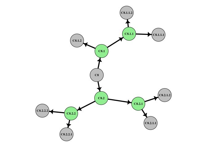
j <- 10 # this changes the target cell and generat different lineage tree
parents <- c()
Offspring <- c()
col <- c()
test <- sub("*\\..d*$", "", unlist(DFF[[j]]))
for (i in 1:length(test)) {
    if (!test[i] == DFF[[j]][i]) {
        parents <- c(parents, test[i])
        Offspring <- c(Offspring, DFF[[j]][i])
    }
}
d <- tibble(Offspring, parents)
d2 <- data.frame(from=d$parents, to=d$Offspring)
g <- graph_from_data_frame(d2)
ordered.vertices <- get.data.frame(g, what="vertices")
for (n in 1:length(parents)) {
    if (Offspring[n] %in% parents) {
        col <- c(col, Offspring[n])
    }
}
COLOR <- c(rep("gray", length(ordered.vertices[, 1])))
for (i in 1:length(ordered.vertices[, 1])) {
    if (ordered.vertices[i, 1] %in% col) {
        COLOR[i] <- "lightgreen"
    }
}
TTT <- TT / TT[which.max(TT)]
E(g)$weight <- TTT
set.seed(100)
test.layout <- layout_(g, with_dh(weight.edge.lengths=TTT))
test.layout[, 1] <- test.layout[, 1] * 2
test.layout[, 2] <- test.layout[, 2] * 3.5
par(mar=c(0, 0,0, 0) + .1)
plot(
    g, layout=test.layout, edge.arrow.size=0.64, edge.arrow.width=2,
    edge.width=3.5, vertex.shape="circle", vertex.size=22, edge.color="black",
    vertex.color=adjustcolor(COLOR, alpha.f=.999), vertex.label.cex=0.65,
    vertex.label.font=2, vertex.label.color="black"
)
df <- read.csv(file.path(path, "PIP-FUCCI All Cells_Results.csv"))
head(df)
dim(df)
mothers <- c()
first <- c()
second <- c()
third <- c()
fourth <- c()
for (i in 1:length(df[, 1])) {
    st <- strsplit(df[i, 3], regex("\\.", multiline=TRUE))
    L <- length(st[[1]]) - 1
    if (L == 0) {mothers=c(mothers, L)}
    if (L == 1) {first=c(first, L)}
    if (L == 2) {second=c(second, L)}
    if (L == 3) {third=c(third, L)}
    if (L == 4) {fourth=c(fourth, L)}
}
generations=c(length(fourth),length(third),length(second),length(first),length(mothers))
barplot(generations,horiz=T,col=c("bisque1","bisque2","bisque3","bisque4", "antiquewhite4"),xlab="Number of cells",xlim=c(0,100))
box()
dcells <- read.csv(file.path(path, "PIP-FUCCI Daughter Cells_Results.csv"))
dim(dcells)
## [1] 118 11
head(dcells)## ExperimentName TiffFileName CellName isDivided isDaughter nImages Distance Displacement TrajectoryTime Directionality
## 1 PIP-FUCCI PIP-FUCCI.tif C1.1 FALSE TRUE 55 82.2 7.4 540 0.089
## 2 PIP-FUCCI PIP-FUCCI.tif C1.2 FALSE TRUE 45 74.2 7.8 440 0.106
## 3 PIP-FUCCI PIP-FUCCI.tif C3.1 TRUE TRUE 123 178.1 27.7 1220 0.156
## 4 PIP-FUCCI PIP-FUCCI.tif C3.1.1 TRUE TRUE 113 127.2 40.5 1120 0.319
## 5 PIP-FUCCI PIP-FUCCI.tif C3.1.1.1 FALSE TRUE 48 72.9 19.3 470 0.265
## 6 PIP-FUCCI PIP-FUCCI.tif C3.1.1.2 FALSE TRUE 51 74.6 11.1 500 0.148
## AverageSpeed
## 1 0.152
## 2 0.169
## 3 0.146
## 4 0.114
## 5 0.155
## 6 0.149
implode <- function(..., sep='') {
     paste(..., collapse=sep)
}
newDF1<-data.frame()
for (i in 1: length(dcells[,1])){
    w<-strsplit(dcells[i,3], "")
    ww<-w[[1]][length(w[[1]])]
    ww<-as.numeric(w[[1]][length(w[[1]])])
    if (ww==1){
        w[[1]][length(w[[1]])]<-2
        se<-implode(w[[1]])
        wh<-which(dcells[,3]==paste0(se))
        if (length(wh)>0){
            newDF1<-rbind(newDF1,dcells[i,],dcells[wh,])
        }
    }
}

dcells<-newDF1
head(dcells)
## ExperimentName TiffFileName CellName isDivided isDaughter nImages Distance Displacement TrajectoryTime Directionality
## 1 PIP-FUCCI PIP-FUCCI.tif C1.1 FALSE TRUE 55 82.2 7.4 540 0.089
## 2 PIP-FUCCI PIP-FUCCI.tif C1.2 FALSE TRUE 45 74.2 7.8 440 0.106
## 3 PIP-FUCCI PIP-FUCCI.tif C3.1 TRUE TRUE 123 178.1 27.7 1220 0.156
## 10 PIP-FUCCI PIP-FUCCI.tif C3.2 TRUE TRUE 133 181.2 9.8 1320 0.054
## 4 PIP-FUCCI PIP-FUCCI.tif C3.1.1 TRUE TRUE 113 127.2 40.5 1120 0.319
## 7 PIP-FUCCI PIP-FUCCI.tif C3.1.2 TRUE TRUE 126 126.7 32.0 1250 0.253
## AverageSpeed
## 1 0.152
## 2 0.169
## 3 0.146
## 10 0.137
## 4 0.114
## 7 0.101
firstDC <- c() # selecting first DCell
num <- c(1:length(dcells[, 1]))
for (k in num) {
    if(!(k %% 2) == 0) {
        firstDC <- c(firstDC, k)
    }
}

sdDiff <- 15  # no trajectory time difference larger than 2.5 hours between the two daughter cells
minStep <- 36 # minimum trajectory time of 6 hours

selectedrows <- c()
for (i in firstDC) {
    condition1 <- abs(dcells[i, 6] - dcells[i + 1, 6]) <= sdDiff
    condition2 <- dcells[i, 6] >= minStep
    condition3 <- dcells[i + 1, 6] >= minStep
    if (condition1 & condition2 & condition3) {
        selectedrows <- c(selectedrows, i)
    }
}

Fselectedrows <- c(selectedrows, (selectedrows + 1)) # including the other cell
Fselectedrows <- sort(Fselectedrows)
Fdcells <- dcells[Fselectedrows, ]
diffDC <- dcells[selectedrows, ]
for (i in selectedrows) {
    diffDC[which(selectedrows %in% i), 5:11] <- abs(
        dcells[i, 5:11] - dcells[i + 1, 5:11]
    )
}
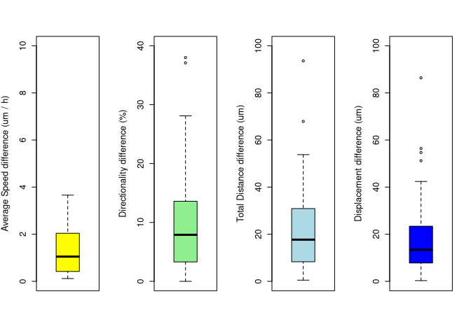
length(diffDC[, 1])         # pairs of daughter cells included in the analysis
## [1] 34
summary(diffDC[, 11] * 60) # speed difference## Min. 1st Qu. Median Mean 3rd Qu. Max.
## 0.120 0.420 1.050 1.346 2.010 3.660
summary(diffDC[, 7]) # total distance difference## Min. 1st Qu. Median Mean 3rd Qu. Max.
## 0.500 8.325 17.700 23.074 30.800 93.600
summary(diffDC[, 10] * 100) # directionality difference (%)## Min. 1st Qu. Median Mean 3rd Qu. Max.
## 0.00 3.35 7.90 10.73 13.32 38.00
summary(diffDC[, 8]) # displacement difference## Min. 1st Qu. Median Mean 3rd Qu. Max.
## 0.30 7.90 13.40 18.68 23.07 86.40
par(mfrow=c(1, 4))
boxplot(
    diffDC[, 11] * 60, ylab="Average Speed difference (um / h)", cex.lab=1.2,
    cex.axis=1.2, col="yellow", ylim=c(0, 10)
)
boxplot(
    diffDC[, 10] * 100, ylab="Directionality difference (%)", cex.lab=1.2,
    cex.axis=1.2, col="lightgreen", ylim=c(0, 40)
)
boxplot(
    diffDC[, 7], ylab="Total Distance difference (um)", cex.lab=1.2,
    cex.axis=1.2, col="lightblue", ylim=c(0, 100)
)
boxplot(
    diffDC[, 8], ylab="Displacement difference (um)", cex.lab=1.2,
    cex.axis=1.2, col="blue", ylim=c(0, 100)
)
TimeDifferences <- c()
for (i in firstDC) {
    if (dcells[i, 4] == TRUE & dcells[i + 1, 4] == TRUE) {
        h <- abs(dcells[i, 9] - dcells[i + 1, 9])
        TimeDifferences <- c(TimeDifferences, h)
    }
}
length(TimeDifferences) # pairs of daughter cells included in the analysis
## [1] 20
summary(TimeDifferences / 60)## Min. 1st Qu. Median Mean 3rd Qu. Max.
## 0.3333 1.1250 1.7500 3.5167 3.8750 21.6667
sd(TimeDifferences / 60)## [1] 4.812842
getmode <- function(v) {
    uniqv <- unique(v)
    uniqv[which.max(tabulate(match(v, uniqv)))]
}
result <- getmode(TimeDifferences)
cat("The mode Time Differences till cell division between daughter cells is ",result/60,"\n" )
## The mode Time Differences till cell division between daughter cells is 1.5
boxplot(
    TimeDifferences / 60,
    ylab="Time difference between the division of daughter cells (h)",
    cex.lab=1.2, cex.axis=1.2, col="gray", ylim=c(0, 15), las=1
)
TD <- TimeDifferences / 60
Group <- c(rep(1, length(TD)))
Da <- data.frame(TD, Group)
data_summary <- function(x) {
    m <- mean(x)
    ymin <- m - sd(x)
    ymax <- m + sd(x)
    return(c(y=m, ymin=ymin, ymax=ymax))
}
p <- ggplot(Da, aes(x=Group, y=TD)) +
    geom_violin(trim=FALSE, fill="gray") +
    geom_point(size=2.5, color="black")
p + stat_summary(fun.data=data_summary, geom="pointrange", color="red", size=1)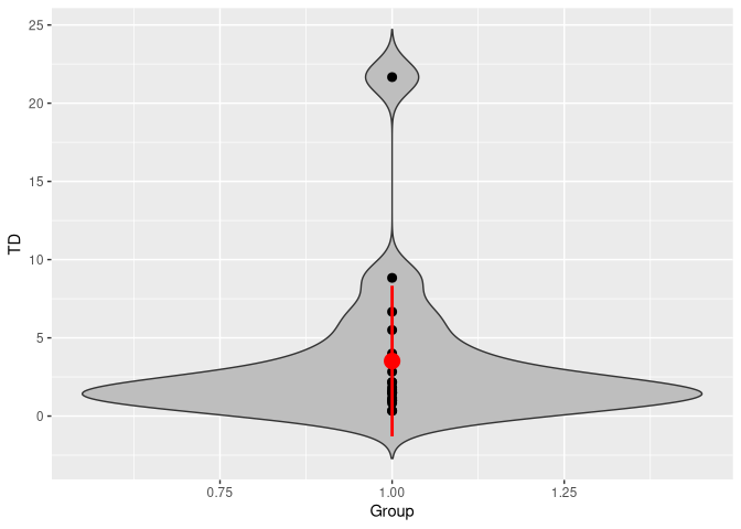
dff <- read.csv(
    file.path(path, "RPE_FUCCI_cell-cycle_dividing_daughter_cells.csv")
)
dim(dff)
## [1] 6245 9
head(dff)## CellID CellName ImageID Xpos Ypos Red Green Blue CyclePhase
## 1 3 C3.1 33 741 134 29.75614 18.697543 16.83932
## 2 3 C3.1 34 742 122 25.00000 9.761815 15.20605
## 3 3 C3.1 35 739 122 24.33459 8.147448 16.06049
## 4 3 C3.1 36 738 126 22.77694 7.502836 15.11153
## 5 3 C3.1 37 740 123 20.14556 7.334594 13.43100
## 6 3 C3.1 38 734 122 21.99244 6.516068 13.86957
pixel_size <- 0.65Cells <- subset(dff, dff[, 9] != "") # removing rows with NA
dim(Cells)## [1] 5601 9
row.has.na <- apply(Cells, 1, function(x) {any(is.na(x))}) # check if rows NAs
Cells <- Cells[!row.has.na, ]
dim(Cells)
## [1] 5601 9
Cells [, 4] <- Cells [, 4] * pixel_size
Cells [, 5] <- Cells [, 5] * pixel_size
SP1 <- split(Cells, Cells[, 2]) # splitting cells based on their ID
length(SP1) # getting the number of dividing daughter cells
## [1] 43
for (u in 1:length(SP1)) {
    SP1[[u]] <- split(SP1[[u]], SP1[[u]][, 9]) # split each cell based on phases
}G1 <- c()
G2 <- c()
S <- c()
for (p in 1:length(SP1)) {
denominator <- sum(
length(SP1[[p]][[1]][, 1]),
length(SP1[[p]][[2]][, 1]),
length(SP1[[p]][[3]][, 1])
)
g1 <- length(SP1[[p]][[1]][, 1]) / denominator
g2 <- length(SP1[[p]][[2]][, 1]) / denominator
s <- length(SP1[[p]][[3]][, 1]) / denominator
G1 <- c(G1, g1)
G2 <- c(G2, g2)
S <- c(S, s)
}
mG1 <- round(mean(G1) * 100)
sdG1 <- round(sd(G1) * 100)
mS <- round(mean(S) * 100)
sdS <- round(sd(S) * 100)
mG2 <- round(mean(G2) * 100)
sdG2 <- round(sd(G2) * 100)yy <- c(mG1, mS, mG2)
std1 <- c(sdG1, sdS, sdG2)
pp <- barplot(
yy, ylim=c(0, 100), xlab="Cell cycle phases",
ylab="Phase average length (%)", las=1, names.arg=c("G1", "S", "G2"),
col=c("khaki2", "khaki3", "khaki4")
)
segments(pp, yy-std1, pp, yy + std1)
segments(pp - 0.1, yy - std1, pp + 0.1, yy - std1)
segments(pp - 0.1, yy + std1, pp + 0.1, yy + std1)
box()
y <- c(G2, S, G1)
Group <- factor(
    c(rep("G1", 43), rep("S", 43), rep("G2", 43)), levels=c("G1", "S", "G2")
)
Group <- factor(Group, levels=c("G1", "S" ,"G2")) # define display order
df <- data.frame(y, Group)
kruskal.test(y ~ Group, data=df)
##
## Kruskal-Wallis rank sum test
##
## data: y by Group
## Kruskal-Wallis chi-squared = 83.538, df = 2, p-value < 2.2e-16
pairwise.wilcox.test(y, Group, p.adj="none", exact=FALSE)##
## Pairwise comparisons using Wilcoxon rank sum test with continuity correction
##
## data: y and Group
##
## G1 S
## S 1.5e-15 -
## G2 0.24 1.0e-14
##
## P value adjustment method: none
TimeInterval <- 10
for (p in 1:length(SP1)) {
    for (v in 1:3) {
        M <- SP1[[p]][[v]]
        MM <- length(M[, 1])
        res <- t(
            sapply(
                1:MM,
                function(i) {
                    # creating values for dx
                    SP1[[p]][[v]][i, 10] <- (SP1[[p]][[v]][i + 1, 4]) -
                        (SP1[[p]][[v]][i, 4])
                    SP1[[p]][[v]][, 10][is.na(SP1[[p]][[v]][, 10])] <- 0
                    # creating values for dy
                    SP1[[p]][[v]][i, 11] <- (SP1[[p]][[v]][i + 1, 5]) -
                        (SP1[[p]][[v]][i, 5])
                    # to remove NA and replace it with 0
                    SP1[[p]][[v]][, 11][is.na(SP1[[p]][[v]][, 11])] <- 0
                    # creating values for dis
                    SP1[[p]][[v]][i, 12] <- sqrt((SP1[[p]][[v]][i, 10]) ^ 2 +
                        (SP1[[p]][[v]][i, 11]) ^ 2)
                    # creating values for Square Speed
                    SP1[[p]][[v]][i, 13] <-
                        ((SP1[[p]][[v]][i, 12]) / TimeInterval) * 60
                    return(SP1[[p]][[v]][i, c(10:13)])
                }
            )
        )
        SP1[[p]][[v]][1:MM, c(10:13)] <- as.data.frame(res)
        SP1[[p]][[v]][, c(10:13)] <- lapply(
            SP1[[p]][[v]][, c(10:13)], as.numeric
        )
        colnames(SP1[[p]][[v]]) <- c(
            "CellID", "CellName", "ImageID", "X", "Y", "R", "G", "B", "phase",
            "dX", "dY", "Dis", "Speed"
        )
    }
}speedG1 <- c()
speedG2 <- c()
speedS <- c()
for (p in 1:length(SP1)) {
sG1 <- mean(SP1[[p]][[1]][, 13])
speedG1 <- c(speedG1, sG1)
sG2 <- mean(SP1[[p]][[2]][, 13])
speedG2 <- c(speedG2, sG2)
sS <- mean(SP1[[p]][[3]][, 13])
speedS <- c(speedS, sS)
}
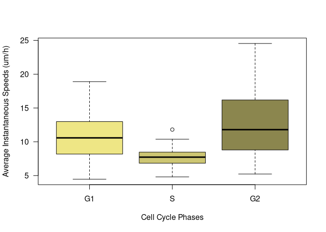
summary(speedG1)## Min. 1st Qu. Median Mean 3rd Qu. Max.
## 4.461 8.183 10.579 10.818 12.985 18.898
sd(speedG1)## [1] 3.668529
summary(speedS)## Min. 1st Qu. Median Mean 3rd Qu. Max.
## 4.812 6.828 7.729 7.758 8.471 11.806
sd(speedS)## [1] 1.551162
summary(speedG2)## Min. 1st Qu. Median Mean 3rd Qu. Max.
## 5.233 8.794 11.794 12.620 16.187 24.540
sd(speedG2)## [1] 4.40839
x1 <- speedG1
x2 <- speedS
x3 <- speedG2plot(1, 1, xlim = c(0, 4), ylim = c(0, 30), type = 'n', xlab = 'Cell Cycle Phases', ylab = '', xaxt = 'n',las=1)
vioplot(x1, at=1, add=TRUE, col="khaki2")
vioplot(x2, at=2, add=TRUE, col="khaki3")
vioplot(x3, at=3, add=TRUE, col="khaki4")
axis(1, at=c(1, 2,3), labels=c('G1', "S", "G2"))
axis(2, at =30, pos=-0.45, tck=0, labels='Average Instantaneous Speeds (um/h)')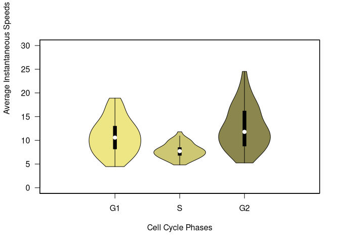
speed <- c(speedG1, speedS, speedG2)
phases <- factor(
    c(rep("G1", 43), rep("S", 43), rep("G2", 43)), levels=c("G1", "S",  "G2")
)
myDF <- data.frame(speed, phases)
boxplot(
    speed ~ phases, data=myDF, las=1, col=c("khaki2", "khaki3", "khaki4"),
    ylab="Average Instantaneous Speeds (um/h)", xlab="Cell Cycle Phases"
)
msG1 <- mean(speedG1)
sdG1 <- sd(speedG1)
msS <- mean(speedS)
sdS <- sd(speedS)
msG2 <- mean(speedG2)
sdG2 <- sd(speedG2)
yy <- c(msG1, msS, msG2)
std1 <- c(sdG1, sdS, sdG2)
pp<-barplot(yy,ylim=c(0,30),xlab="Cell cycle phases",ylab="Average Instantaneous Speeds (um/h)",las=1,names.arg=c("G1","S","G2"),col = c("khaki2","khaki3","khaki4"))
segments(pp, yy - std1, pp, yy + std1)
segments(pp - 0.1, yy - std1, pp + 0.1, yy - std1)
segments(pp - 0.1, yy + std1, pp + 0.1, yy + std1)
box()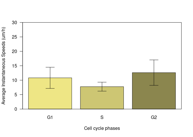
y <- c(speedG1, speedS, speedG2)
Group <- factor(
    c(rep("G1", 43), rep("S", 43), rep("G2", 43)), levels=c("G1", "S",  "G2")
)
Group <- factor(Group, levels=c("G1", "S" ,"G2")) # order to be displayed
df <- data.frame(y, Group)
kruskal.test(y ~ Group, data=df)
##
## Kruskal-Wallis rank sum test
##
## data: y by Group
## Kruskal-Wallis chi-squared = 36.436, df = 2, p-value = 1.225e-08
pairwise.wilcox.test(y, Group, p.adj="none", exact=FALSE)##
## Pairwise comparisons using Wilcoxon rank sum test with continuity correction
##
## data: y and Group
##
## G1 S
## S 2.8e-05 -
## G2 0.094 5.5e-09
##
## P value adjustment method: none
disG1 <- c()
displacementG1 <- c()
disG2 <- c()
displacementG2 <- c()
disS <- c()
displacementS <- c()
for (p in 1:length(SP1)) {
    sG1 <- sum(SP1[[p]][[1]][, 12])
    disG1 <- c(disG1, sG1)
    dG1 <- sqrt(
        (SP1[[p]][[1]][length(SP1[[p]][[1]][, 1]), 4] - SP1[[p]][[1]][1, 4])^2 +
        (SP1[[p]][[1]][length(SP1[[p]][[1]][, 1]), 5] - SP1[[p]][[1]][1, 5])^2
    )
    displacementG1 <- c(displacementG1, dG1)

    sG2 <- sum(SP1[[p]][[2]][, 12])
    disG2 <- c(disG2, sG2)
    dG2 <- sqrt(
        (SP1[[p]][[2]][length(SP1[[p]][[2]][, 1]), 4] - SP1[[p]][[2]][1, 4])^2 +
        (SP1[[p]][[2]][length(SP1[[p]][[2]][, 1]), 5] - SP1[[p]][[2]][1, 5])^2
    )
    displacementG2 <- c(displacementG2, dG2)

    sS <- sum(SP1[[p]][[3]][, 12])
    disS <- c(disS, sS)
    dS <- sqrt(
        (SP1[[p]][[3]][length(SP1[[p]][[3]][, 1]), 4] - SP1[[p]][[3]][1, 4])^2 +
        (SP1[[p]][[3]][length(SP1[[p]][[3]][, 1]), 5] - SP1[[p]][[3]][1, 5])^2
    )
    displacementS <- c(displacementS, dS)
}

DRg1 <- displacementG1 / disG1
DRg2 <- displacementG2 / disG2
DRs <- displacementS / disS
mean(DRg1)
## [1] 0.2274437
sd(DRg1)## [1] 0.1563529
mean(DRs)## [1] 0.205804
sd(DRg2)## [1] 0.171562
mean(DRg2)## [1] 0.2862626
sd(DRg2)## [1] 0.171562
DIS <- c(DRg1, DRs, DRg2)
phases <- factor(
    c(rep("G1", 43), rep("S", 43), rep("G2", 43)), levels=c("G1", "S",  "G2")
)
myDF <- data.frame(DIS, phases)
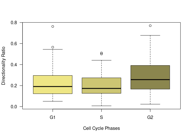
boxplot(
    DIS ~ phases, data=myDF, las=1, col=c("khaki2", "khaki3", "khaki4"),
    ylab="Directionality Ratio", xlab="Cell Cycle Phases"
)
msG1 <- mean(DRg1)
sdG1 <- sd(DRg1)
msS <- mean(DRs)
sdS <- sd(DRs)
msG2 <- mean(DRg2)
sdG2 <- sd(DRg2)
yy <- c(msG1, msS, msG2)
std1 <- c(sdG1, sdS, sdG2)
pp <- barplot(
    yy, ylim=c(0, 0.6), xlab="Cell cycle phases", ylab="Directionality", las=1,
    names.arg=c("G1", "S", "G2"), col=c("khaki2", "khaki3", "khaki4")
)
segments(pp, yy - std1, pp, yy + std1)
segments(pp - 0.1, yy - std1, pp + 0.1, yy - std1)
segments(pp - 0.1, yy + std1, pp + 0.1, yy + std1)
box()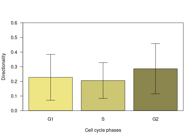
y <- c(DRg1, DRs, DRg2)
Group <- factor(
    c(rep("G1", 43), rep("S", 43), rep("G2", 43)), levels=c("G1", "S",  "G2")
)
Group <- factor(Group, levels=c("G1", "S" ,"G2")) # order to be displayed
df <- data.frame(y, Group)
kruskal.test(y ~ Group, data=df)
##
## Kruskal-Wallis rank sum test
##
## data: y by Group
## Kruskal-Wallis chi-squared = 5.8015, df = 2, p-value = 0.05498
pairwise.wilcox.test(y, Group, p.adj="none", exact=FALSE)##
## Pairwise comparisons using Wilcoxon rank sum test with continuity correction
##
## data: y and Group
##
## G1 S
## S 0.660 -
## G2 0.081 0.020
##
## P value adjustment method: none
SP2 <- split(Cells, Cells[, 2]) # splitting each cell based on phases
TimeInterval <- 10
for (p in 1:length(SP2)) {
    M <- SP2[[p]]
    MM <- length(M[, 1])
    res <- t(
        sapply(
            1:MM,
            function(i) {
                # creating values for dx
                SP2[[p]][i, 10] <- (SP2[[p]][i + 1, 4]) - (SP2[[p]][i, 4])
                SP2[[p]][, 10][is.na(SP2[[p]][, 10])] <- 0
                # creating values for dy
                SP2[[p]][i, 11] <- (SP2[[p]][i + 1, 5]) - (SP2[[p]][i, 5])
                # to remove NA and replace it with 0
                SP2[[p]][, 11][is.na(SP2[[p]][, 11])] <- 0
                # creating values for dis
                SP2[[p]][i, 12] <- sqrt(
                    (SP2[[p]][i, 10]) ^ 2 + (SP2[[p]][i, 11]) ^ 2
                )
                # creating values for Square Speed
                SP2[[p]][i, 13] <- ((SP2[[p]][i, 12])/TimeInterval) * 60
                return(SP2[[p]][i, c(10:13)])
            }
        )
    )
    SP2[[p]][1:MM, c(10:13)] <- as.data.frame(res)
    SP2[[p]][, c(10:13)] <- lapply(SP2[[p]][, c(10:13)], as.numeric)
    colnames(SP2[[p]]) <- c(
        "CellID", "CellName", "ImageID", "X", "Y", "R", "G", "B", "Phase",
        "dX", "dY", "Dis", "Speed"
    )
}time <- c(1:144)
length(time)## [1] 144
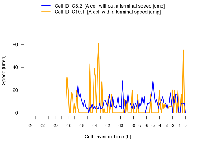
# An example of a cell with a jump
i <- 1
x <- c(
    1, 6,12, 18, 24, 30, 36, 42, 48, 54, 60, 66, 72, 78, 84, 90, 96, 102, 108,
    114, 120, 126, 132, 138, 144
)
y <- c(
    -24, -23, -22, -21, -20, -19, -18, -17, -16, -15, -14, -13, -12, -11, -10,
    -9, -8, -7, -6, -5, -4, -3, -2, -1, 0
)

if (length(SP2[[i]][, 13]) <= 144) {
    missing <- 144 - length(SP2[[i]][, 13])
    P <- c(rep(NA, missing), SP2[[i]][, 13])
    length(P)
    plot(time,P,type="l", lwd=3,col="orange",ylim=c(0,75),xaxt="n", xlab="Cell Division Time (h)",ylab="Speed (um/h)",las=1)
    axis(1, at=x, labels=y, col.axis="black", cex.axis=0.73, las=1)
} else {
    extra <- 144 - length(SP2[[i]][, 13])
    P <- SP2[[i]][(1 + abs(extra)):length(SP2[[i]][, 13]), 13]
    plot(time,P,type="l", lwd=3,col="red",ylim=c(0,75),xaxt="n", xlab="Cell Division Time (h)",ylab="Speed (um/h)",las=1)
    axis(1, at=x, labels=y, col.axis="black", las=1)
}

# An example of a cell without a jump
i <- 35
missing <- 144 - length(SP2[[i]][, 13])
P <- c(rep(NA, missing), SP2[[i]][, 13])
lines(time, P, lwd=2.2, col="blue")
add_legend <- function(...) {
    opar <- par(
        fig=c(0, 1, 0, 1), oma=c(0, 0, 0, 0), mar=c(0, 0, 0, 0), new=TRUE
    )
    on.exit(par(opar))
    plot(0, 0, type='n', bty='n', xaxt='n', yaxt='n')
    legend(...)
}
add_legend(
    "top",
    legend=c(
        "Cell ID: C8.2  [A cell without a terminal speed jump]",
        "Cell ID: C10.1  [A cell with a terminal speed jump]"
    ),
    col=c("blue", "orange"), horiz=FALSE, bty='n', cex=1, lty=1, lwd=2.4
)
SP2 <- split(Cells, Cells[, 2]) # splitting each cell based on phases
TimeInterval <- 5
for (p in 1:length(SP2)) {
    M <- SP2[[p]]
    MM <- length(M[, 1])
    res <- t(
        sapply(
            1:MM,
            function(i) {
                # creating values for dx
                SP2[[p]][i, 10] <- (SP2[[p]][i + 1, 4]) - (SP2[[p]][i, 4])
                SP2[[p]][, 10][is.na(SP2[[p]][, 10])] <- 0
                # creating values for dy
                SP2[[p]][i, 11] <- (SP2[[p]][i + 1, 5]) - (SP2[[p]][i, 5])
                # to remove NA and replace it with 0
                SP2[[p]][, 11][is.na(SP2[[p]][, 11])] <- 0
                # creating values for dis
                SP2[[p]][i, 12] <- sqrt(
                    (SP2[[p]][i, 10]) ^ 2 + (SP2[[p]][i, 11]) ^ 2
                )
                # creating values for Square Speed
                SP2[[p]][i, 13] <- ((SP2[[p]][i, 12]) / TimeInterval) * 60
                return(SP2[[p]][i, c(10:13)])
            }
        )
    )
    SP2[[p]][1:MM, c(10:13)] <- as.data.frame(res)
    SP2[[p]][, c(10:13)] <- lapply(SP2[[p]][, c(10:13)], as.numeric)
    colnames(SP2[[p]]) <- c(
        "CellID", "CellName", "ImageID", "X", "Y", "R", "G", "B", "Phase",
        "dX", "dY", "Dis", "Speed"
    )
}

jump <- c()
for(i in 1:length(SP2)) {
    if (length(SP2[[i]][, 13]) < 144) {
        missing <- 144 - length(SP2[[i]][, 13])
        SP2[[i]][1:144, 13] <- c(rep(NA, missing), SP2[[i]][, 13])
    } else {
        extra <- 144 - length(SP2[[i]][, 13])
        SP2[[i]][1:144, 13] <- SP2[[i]][(1 + abs(extra)):length(SP2[[i]][, 13]), 13]
    }
    testB <- SP2[[i]][138:144, 13]
    testA <- SP2[[i]][130:137, 13]
    condition1 <- mean(testB[testB != 0])> mean(testA[testA != 0]) * 1.5
    if (condition1 & ((SP2[[i]][138, 13])>= 2.5 * mean(SP2[[i]][120:144, 13])) & ((SP2[[i]][138, 13])>= (3 * SP2[[i]][140, 13])| (SP2[[i]][138, 13])>= (3 * SP2[[i]][141, 13]) | (SP2[[i]][138, 13])>= (3 * SP2[[i]][142, 13])| (SP2[[i]][138, 13])>= (3 * SP2[[i]][139, 13]) | (SP2[[i]][138, 13])>= (3 * SP2[[i]][144, 13])| (SP2[[i]][138, 13])>= (3 * SP2[[i]][143, 13]))) {
        jump <- c(jump, i)}
    if (condition1 & ((SP2[[i]][139, 13])>= 2.5 * mean(SP2[[i]][120:144, 13])) & ((SP2[[i]][139, 13])>= (3 * SP2[[i]][140, 13])| (SP2[[i]][139, 13])>= (3 * SP2[[i]][141, 13]) | (SP2[[i]][139, 13])>= (3 * SP2[[i]][142, 13])| (SP2[[i]][139, 13])>= (3 * SP2[[i]][138, 13]) | (SP2[[i]][139, 13])>= (3 * SP2[[i]][144, 13])| (SP2[[i]][139, 13])>= (3 * SP2[[i]][143, 13]))) {
        jump <- c(jump, i)}
    if (condition1 & ((SP2[[i]][140, 13])>= 2.5 * mean(SP2[[i]][120:144, 13])) & ((SP2[[i]][140, 13])>= (3 * SP2[[i]][138, 13])| (SP2[[i]][140, 13])>= (3 * SP2[[i]][141, 13]) | (SP2[[i]][140, 13])>= (3 * SP2[[i]][142, 13])| (SP2[[i]][140, 13])>= (3 * SP2[[i]][139, 13]) | (SP2[[i]][140, 13])>= (3 * SP2[[i]][144, 13])| (SP2[[i]][140, 13])>= (3 * SP2[[i]][143, 13]))) {
        jump <- c(jump, i)}
    if (condition1 & ((SP2[[i]][141, 13])>= 2.5 * mean(SP2[[i]][120:144, 13])) & ((SP2[[i]][141, 13])>= (3 * SP2[[i]][140, 13])| (SP2[[i]][141, 13])>= (3 * SP2[[i]][138, 13]) | (SP2[[i]][141, 13])>= (3 * SP2[[i]][142, 13])| (SP2[[i]][141, 13])>= (3 * SP2[[i]][139, 13]) | (SP2[[i]][141, 13])>= (3 * SP2[[i]][144, 13])| (SP2[[i]][141, 13])>= (3 * SP2[[i]][143, 13]))) {
        jump <- c(jump, i)}
    if (condition1  & ((SP2[[i]][142, 13])>= 2.5 * mean(SP2[[i]][120:144, 13]))& ((SP2[[i]][142, 13])>= (3 * SP2[[i]][140, 13])| (SP2[[i]][142, 13])>= (3 * SP2[[i]][141, 13]) | (SP2[[i]][142, 13])>= (3 * SP2[[i]][138, 13])| (SP2[[i]][142, 13])>= (3 * SP2[[i]][139, 13]) | (SP2[[i]][142, 13])>= (3 * SP2[[i]][144, 13])| (SP2[[i]][142, 13])>= (3 * SP2[[i]][143, 13]))) {
        jump <- c(jump, i)}

    if (condition1 & ((SP2[[i]][143, 13])>= 2.5 * mean(SP2[[i]][120:144, 13])) & ((SP2[[i]][143, 13])>= (3 * SP2[[i]][140, 13])| (SP2[[i]][143, 13])>= (3 * SP2[[i]][141, 13]) | (SP2[[i]][143, 13])>= (3 * SP2[[i]][142, 13])| (SP2[[i]][143, 13])>= (3 * SP2[[i]][139, 13]) | (SP2[[i]][143, 13])>= (3 * SP2[[i]][144, 13])| (SP2[[i]][143, 13])>= (3 * SP2[[i]][138, 13]))) {
        jump <- c(jump, i)}
    if (condition1 & ((SP2[[i]][144, 13])>= 2.5 * mean(SP2[[i]][120:144, 13])) & ((SP2[[i]][144, 13])>= (3 * SP2[[i]][140, 13])| (SP2[[i]][144, 13])>= (3 * SP2[[i]][141, 13]) | (SP2[[i]][144, 13])>= (3 * SP2[[i]][142, 13])| (SP2[[i]][144, 13])>= (3 * SP2[[i]][143, 13]) | (SP2[[i]][144, 13])>= (3 * SP2[[i]][139, 13])| (SP2[[i]][144, 13])>= (3 * SP2[[i]][138, 13]))) {
        jump <- c(jump, i)}
    if (mean(testB[testB != 0])> 5 * (mean(testA[testA != 0]))) {
        jump <- c(jump, i)
    }
    jump <- jump[!duplicated(jump)]
}

length(jump) # number of cells with a jump
## [1] 35
(length(jump) / length(SP2)) * 100 # % of cells with a jump## [1] 81.39535
jumpDF <- data.frame()
for (j in jump) {
    jumpDF <- rbind(jumpDF, SP2[[j]][, 13])
}
dim(jumpDF)
## [1] 35 144
nam <- c(1:144)
colnames(jumpDF) <- nam
for (i in 1:144) {
    jumpDF[length(jump) + 1, i]<- mean(jumpDF[1:length(jump), i], na.rm=TRUE)
    jumpDF[length(jump) + 2, i]<- sd(jumpDF[1:length(jump), i], na.rm=TRUE)
}
x <- time
y <- jumpDF[length(jump) + 1, ]
dy <- jumpDF[length(jump) + 2, ]
Time <- x
p <- graphics::plot(
    Time, y, type="l", col="red", xaxt="n", xlab="Cell Division Time (h)",
    ylab="Speed (um/h)", lwd=1, las=1, ylim=c(0, 220)
)
graphics::polygon(
    c(Time, rev(Time)), c(y + dy, rev(y-dy)), col="gray" , border=NA
)
graphics::lines(Time, y + dy, col="black")
graphics::lines(Time, y - dy, col="black")
graphics::lines(Time, y, type="l", col="red", lwd=3)
xx=c(1,6,12,18,24,30,36,42,48,54,60,66,72,78,84,90,96,102,108,114,120,126,132,138,144)
yy=c(-24,-23,-22,-21,-20,-19,-18,-17,-16,-15,-14,-13,-12,-11,-10,-9,-8,-7,-6,-5,-4,-3,-2,-1,0)
axis(1, at=xx, labels=yy, col.axis="black", las=1, cex.axis=0.73)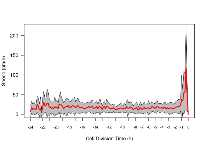
SP2 <- split(Cells, Cells[, 2]) # splitting each cell based on phases
TimeInterval <- 10
for (p in 1:length(SP2)) {
    M <- SP2[[p]]
    MM <- length(M[, 1])
    res <- t(
        sapply(
            1:MM,
            function(i) {
                # creating values for dx
                SP2[[p]][i, 10] <- (SP2[[p]][i + 1, 4]) - (SP2[[p]][i, 4])
                SP2[[p]][, 10][is.na(SP2[[p]][, 10])] <- 0
                # creating values for dy
                SP2[[p]][i, 11] <- (SP2[[p]][i + 1, 5]) - (SP2[[p]][i, 5])
                # to remove NA and replace it with 0
                SP2[[p]][, 11][is.na(SP2[[p]][, 11])] <- 0
                # creating values for dis
                SP2[[p]][i, 12] <- sqrt(
                    (SP2[[p]][i, 10]) ^ 2 + (SP2[[p]][i, 11]) ^ 2
                )
                # creating values for Square Speed
                SP2[[p]][i, 13] <- ((SP2[[p]][i, 12]) / TimeInterval) * 60
                return(SP2[[p]][i, c(10:13)])
            }
        )
    )
    SP2[[p]][1:MM, c(10:13)] <- as.data.frame(res)
    SP2[[p]][, c(10:13)] <- lapply(SP2[[p]][, c(10:13)], as.numeric)
    colnames(SP2[[p]]) <- c(
        "CellID", "CellName", "ImageID", "X", "Y", "R", "G", "B", "Phase",
        "dX", "dY", "Dis", "Speed"
    )
}

Total <- c(1:length(SP2))
noJump <- !is.element(Total, jump)
noJump <- Total[noJump]

for(i in 1:length(SP2)) {
    if (length(SP2[[i]][, 13]) < 144) {
        missing <- 144 - length(SP2[[i]][, 13])
        SP2[[i]][1:144, 13] <- c(rep(0, missing), SP2[[i]][, 13])
    } else {
        extra <- 144 - length(SP2[[i]][, 13])
        SP2[[i]][1:144, 13] <- SP2[[i]][(1 + abs(extra)):length(SP2[[i]][, 13]), 13]
    }
}

NOTjumpDF <- data.frame()
for (j in noJump) {
    NOTjumpDF <- rbind(NOTjumpDF, SP2[[j]][, 13])
}
dim(NOTjumpDF)
## [1] 8 144
nam <- c(1:144)
colnames(NOTjumpDF) <- nam
for (i in 1:144) {
    NOTjumpDF[length(noJump) + 1, i] <- mean(
        NOTjumpDF[1:length(noJump), i], na.rm=TRUE
    )
    NOTjumpDF[length(noJump) + 2, i] <- sd(
        NOTjumpDF[1:length(noJump), i], na.rm=TRUE
    )
}
x <- time
y <- NOTjumpDF[length(noJump) + 1, ]
dy <- NOTjumpDF[length(noJump) + 2, ]
Time <- x

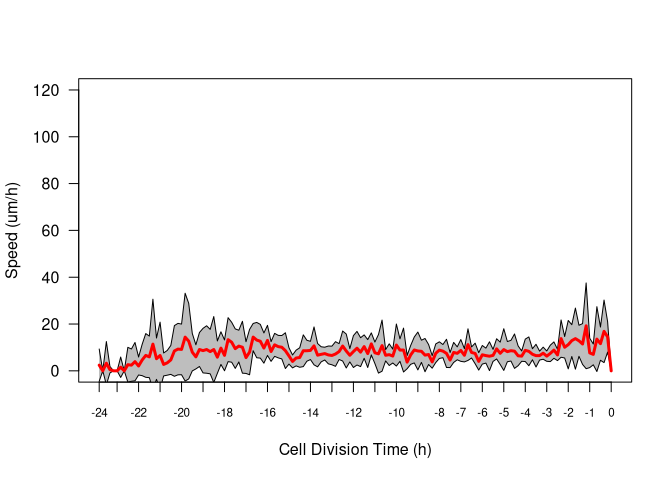
p<-graphics::plot(Time,y, type="l",col="red",xaxt="n",xlab="Cell Division Time (h)",ylab="Speed (um/h)",lwd=1,las=1,ylim=c(0,120))

graphics::polygon(
    c(Time, rev(Time)), c(y + dy, rev(y - dy)), col="gray" , border=NA
)
graphics::lines(Time, y + dy, col="black")
graphics::lines(Time, y - dy, col="black")
graphics::lines(Time, y, type="l", col="red", lwd=3)
xx=c(1,6,12,18,24,30,36,42,48,54,60,66,72,78,84,90,96,102,108,114,120,126,132,138,144)
yy=c(-24,-23,-22,-21,-20,-19,-18,-17,-16,-15,-14,-13,-12,-11,-10,-9,-8,-7,-6,-5,-4,-3,-2,-1,0)
axis(1, at=xx, labels=yy, col.axis="black", las=1, cex.axis=0.73)