Genetic heterogeneity in tumors can show a remarkable selectivity when two or more independent genetic events occur in the same gene. This phenomenon, called composite mutation, points towards to a selective pressure that could cause therapy resistance to mutation-specific drugs. Since composite mutations have been described to occur in sub-clonal populations, they are not always captured through biopsy sampling. Here we provide a proof of concept to predict composite mutations to anticipate which patients might be at risk for sub-clonally driven therapy-resistance. We found that composite mutations occur in 5% of the patients, mostly affecting the PIK3CA, EGFR, BRAF and KRAS genes, which are common drug targets. Furthermore, we found that there is a strong relationship between the frequencies of composite mutations with commonly co-occurring mutations in a non-composite context (p-value 1.7E-10 or lower). We also found that co-mutations frequently occur on the same chromosome (p-values 4.0E-8) and cause a dependency on them (p-value 3.9E-5). The prediction model shows that prediction of compositive mutations is feasible (AUC 0.62, 0.81, 0.82 and 0.91 for EGFR/PIK3CA/KRAS and BRAF), which implicates that our model could help to assess the risk whether patients will develop therapy-resistance against targeted therapies.
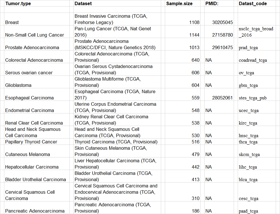
The TCGA source data is available via cbioportal, all source data is retrieved via the cgdsr package. We used the following datasets:
| Tumor.type | Dataset | Sample.size | PMID: | Datast_code |
|---|---|---|---|---|
| Breast | Breast Invasive Carcinoma (TCGA, Firehorse Legacy) | 1108 | 30205045 | |
| Non-Small Cell Lung Cancer | Pan-Lung Cancer (TCGA, Nat Genet 2016) | 1144 | 27158780 | nsclc_tcga_broad_2016 |
| Prostate Adenocarcinoma | Prostate Adenocarcinoma (MSKCC/DFCI, Nature Genetics 2018) | 1013 | 29610475 | prad_tcga |
| Colorectal Adenocarcinoma | Colorectal Adenocarcinoma (TCGA, Provisional) | 640 | NA | coadread_tcga |
| Serous ovarian cancer | Ovarian Serous Cystadenocarcinoma (TCGA, Provisional) | 606 | NA | ov_tcga |
| Glioblastoma | Glioblastoma Multiforme (TCGA, Provisional) | 604 | NA | gbm_tcga |
| Esophageal Carcinoma | Esophageal Carcinoma (TCGA, Nature 2017) | 559 | 28052061 | stes_tcga_pub |
| Endometrial Carcinoma | Uterine Corpus Endometrial Carcinoma (TCGA, Provisional) | 548 | NA | ucec_tcga |
| Renal Clear Cell Carcinoma | Kidney Renal Clear Cell Carcinoma (TCGA, Provisional) | 538 | NA | kirc_tcga |
| Head and Neck Squamous Cell Carcinoma | Head and Neck Squamous Cell Carcinoma (TCGA, Provisional) | 530 | NA | hnsc_tcga |
| Papillary Thyroid Cancer | Thyroid Carcinoma (TCGA, Provisional) | 516 | NA | thca_tcga |
| Cutaneous Melanoma | Skin Cutaneous Melanoma (TCGA, Provisional) | 479 | NA | skcm_tcga |
| Hepatocellular Carcinoma | Liver Hepatocellular Carcinoma (TCGA, Provisional) | 442 | NA | lihc_tcga |
| Bladder Urothelial Carcinoma | Bladder Urothelial Carcinoma (TCGA, Provisional) | 413 | NA | blca_tcga |
| Cervical Squamous Cell Carcinoma | Cervical Squamous Cell Carcinoma and Endocervical Adenocarcinoma (TCGA, Provisional) | 310 | NA | cesc_tcga |
| Pancreatic Adenocarcinoma | Pancreatic Adenocarcinoma (TCGA, Provisional) | 186 | NA | paad_tcga |
 |
Samples with composit mutations (as well as non-composit cases) are shown here: Composite samples
Input data We selected the top four interesting genes with composite mutation based on high frequency and relevance towards targeted therapy (BRAF, EGFR, KRAS, PIK3CA). We divided the data into tumor types that have composite mutations in either BRAF, EGFR, KRAS, or PIK3CA. For all these separated groups we defined all the cases that contain composite mutations or without any composite mutations. Per group of genes with a composite mutation, only the significant co-mutations are taken along as features. These features contain either the information about mutation or copy number variation (binary input) or the distance from co-mutation to the gene with composite mutation (continuous value). All the relative distances of the input belonging to the chromosomal distance model are normalized towards the total distance of the genome (3,000,000,000). See Supplementary Table 2 for all the input data.
Processed Input data for the Random Forest model can be found on the Synapse portal: https://doi.org/10.7303/syn34623212
The R script to create the input can be found here: input_RF_model_geneatlas
The R script for the random forest prediction model can be found here:RF_model_geneatlas
Random Forest The random forest machine learning algorithm was chosen as it is robust and capable of processing high-dimensional datasets. Furthermore, it applies to binary data as well as data containing continuous values. This machine-learning algorithm builds many decision trees, using bagging and feature randomness to create each tree. By combining all these decision trees (an uncorrelated forest of trees) the most accurate prediction is expected in comparison to a single tree. The library randomForestSRC(H. Ishwaran and U.B. Kogalur and E.H. Blackstone and M.S. Lauer 2008) in R is used to build the random forest model with 100 trees. The training set (2/3) and test set(1/3) are created by dividing the data using createDataPartition from the library caret (Max Kuhn 2009). All the default parameters are used for building the model.
Ensemble learning We build separate models for the data for the complementary relationship and the chromosomal disruption. The method of ensemble learning allows us to combine different models to find a more powerful prediction result. We computed a weighted-average prediction ensemble model. The probability score given by the separate random forest models were extracted. As there was a stronger complementary relationship, we multiplied the probability score of this model by 0.75, whereas the chromosomal disruption model was multiplied by 0.25. The highest average score defined the final predictive label. Performance First the false negative (FN), false positive (FP), true negative (TN), and true positive values were defined by comparing the predicted label and the actual label. From there, the true positive rate (TPR), false-positive rate (FPR), sensitivity, specificity, accuracy, and balanced accuracy were calculated (see formula below). The TPR and FPR were plotted to create the receiver operator curve (ROC) as a performance representation of the prediction model. From the ROC we calculated the area under the curve (AUC) values (see formula below). The confusion matrixes contain the TP, TN, FP, and FN.
accuracy=(TN+TP)/(TN+TP+FP+FN)
balanced accuracy=(TP/(TP+FN)+TN/(TN+FP))/2
precision=TP/(TP+FP)
TPR,recall,sensitivity= TP/(TP+FN)
FPR=FP/(TN+FP)
To evaluate our prediction model, we randomly shuffled the features of each dataset from 10 to 100% in 10 steps. From the shuffled data we also build a separate random forest model and got the final prediction for each dataset that has been received after the ensemble learning. For each shuffled data, the performance was calculated and plotted.
The R script for the randomised model can be found here: randomized_RF.R