- Source and Project Code
- Project Introduction and Motivation
- Methods Used
- Project Highlights
- Oliver's Four Factors
- Rule Changes
- Data Cleaning and Exploratory Data Analysis
- Oliver's Four Factors Regression
- Improving the Model
- Tuned Model
- Evaluation of Championship Contenders
- Conclusion
All data was originally found on NBA.com, and I compiled it into a CSV that can be found here. I merged the data from multiple sections the stats page (traditional, advanced, four factors, scoring, opponent) into a single CSV totaling 100 features. All project code can be found here.
Sports are a lifelong passion of mine. I sought out to create a model to predict the number of wins an NBA team would have given specific game-related metrics. As I read more online, I discovered that there has been ample work done covering this problem, notably by basketball statistician Dean Oliver. He is responsible for the creation of the “Four Factors,” an analysis of specific metrics which are thought to be the most important in determining the outcome of a basketball game. With that in mind, I shifted my focus to assess if the Four Factors model is still accurate in today’s era, as well as to try to improve the predictability and/or the insight that could be provided from the model.
All analysis was done in R. Select table and model outputs were reformatted in Excel.
- Descriptive Statistics and Exploratory Data Analysis
- Data Visualization
- Feature Engineering
- Linear Regression
- Scraping and Joining Data (in Excel)
- Assessed the accuracy of Oliver's Four Factors model using linear regression and concluded that the weight of factors should be slightly reallocated (more into shooting)
- Created a model that can more accurately predict (by half a game) how teams will perform through feature engineering weightedpointspershotattempt, a metric that provides more detailed information and better identifies areas to improve
- Model not only performed better on the league-wide level, but also on championship contenders (teams with 50+ wins)
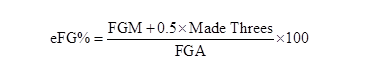
Oliver’s Four Factors are effective field goal %, turnover rate, offensive rebounding percentage, and free throw rate. Each of these metrics can be applied to both opposing teams (effective FG % and opponent’s effective FG %), thus making 8 total factors that are measured.
-
Effective Field Goal Percentage=(Field Goals Made) + (0.5*3P Field Goals Made))/(Field Goal Attempts)
-
Turnover Rate=Turnovers/(Field Goal Attempts + 0.44*Free Throw Attempts + Turnovers)
-
Offensive Rebounding Percentage = (Offensive Rebounds)/[(Offensive Rebounds)+(Opponent’s Defensive Rebounds)]
-
Free Throw Rate=(Free Throws Attempted)/(Field Goals Attempted)
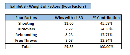
Oliver claims that not all factors are of equal importance, as he applied the following weights to each metric.
- Shooting (40%)
- Turnovers (25%)
- Rebounding (20%)
- Free Throws (15%)
Data was collected from seasons dating back to 2005, at which point in time, a few rule changes had recently been implemented which were influential in the style of play of the modern NBA. A few of the rules are as follows:
1999-00
- A defender may not make contact with his hands and/or forearms on an offensive player except below the free throw line extended.
- A five-second rule that mandates that a player must either shoot, pass or pick up his dribble within five seconds if he begins dribbling the ball with his back toward the basket below the free throw line extended.
2004-05
- New rules were introduced to curtail hand-checking, clarify blocking fouls and call defensive three seconds to open up the game.
These rule changes are certainly influential in the style of play that is seen in the NBA, so I decided to restrict data to 2005 and more recent, with the years 2012 and 2020 being removed due to shortened seasons (lockout and pandemic). Furthermore, 10 years of data was used to train a model (2005-2015 excluding 2012, for a total of 300 observations), and 4 years served as testing data (2016-2019 for a total of 120 observations). More rule changes can be found here.
Variables were renamed for ease of use and uniform notation. The features Team and Team_Season were removed such that factors can be converted to numeric variables, and then these features were added back to the data. Also, ft rate was converted to a percentage to be comparable to other stats.
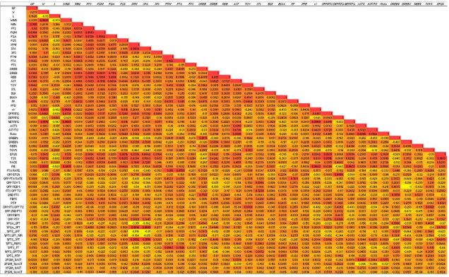
This is a correlation plot made in excel. A similar plot was made in R, but there were too many variables to make for a clear image.
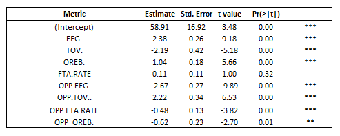
The first test conducted was to perform a linear regression with Oliver’s Four Factors to determine win outcomes. The model proved to be a strong explainer of the relationship, as the following output was produced:
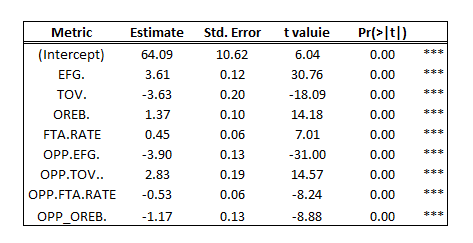
- Adjusted R-Squared = .93
- Residual Standard Error = 3.38 (wins)
The model is well fit to the training data, with an R-Squared value of .93. To determine the accuracy of the model on the testing data, the R-Squared and RMSE values were calculated for the testing set (starting in the 2016 season).
- R2 = 0.91
- RMSE = 3.55 (wins)
- 3.55 Wins / 41 (Mean # of wins) = 8.66%
On average, the predictions were off 3.55 wins (8.66%), indicating that the model was strong in explaining the relationship between the variables.
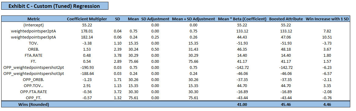
After assessing the influence of each predictor on wins, it was confirmed that this is the correct ranking of importance, however, the weights should be slightly shifted. To determine the appropriate “weight” (or importance) of each factor, factors were assessed based on the change in wins given an increase/decrease in standard deviation. For example, if an increase in one standard deviation of factor A would add 5 wins, and a 1 standard deviation increase in all variables adds 20 total wins, it is concluded that factor A would deserve 25% weight. Absolute values were taken to account for variables that had a negative relationship with wins (i.e. turnovers). Exhibit A displays statistics for each factor such as their mean, standard deviation, and win increase given an increase in standard deviation. For a team with all mean values, their win total would be 41 wins (league average). The Mean + SD adjustment column can be manipulated given team specific stats to understand the impact on wins given a team’s strength/weakness.
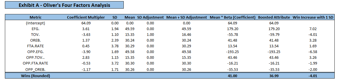 Values are rounded so caluclations may be off
Given the impact of each factor on wins, the following weights have been determined:
- Shooting (45.59%)
- Turnovers (24.36%)
- Rebounding (17.71%)
- Free Throws (12.34%)
It was concluded that Oliver had the correct ranking of importance on each factor, however, the weights should be slightly adjusted. The original weights proposed were 40, 25, 20, 15, and the data suggests some weight be shifted from rebounding and free throws and into shooting. Rule changes over time and player development over decades have largely influenced style of play, and as such, the weights reflect the current NBA (last 15 years). In basketball terms, the win increase potential of a variable can be interpreted through the following example. If a team turns the ball over 1 standard deviation above league average (more often than), and with all other factors held constant, they will lose 4 additional games (Exhibit A). This translates to a team turning the ball over on 16.46% of its possessions rather than 15.35%. The same process can be applied to any of the factors to find how many wins will result from a tweak in a metric. Perhaps what is more subjective is assessing how difficult” it is for a team to manipulate the value of each factor. Even though each factor has a different weight, or “importance”, are all equally easy to adjust? Sure, one standard deviation of EFG% may have a larger impact on the win total than turnovers, but is it easier to raise the EFG% nearly 2%, or turn the ball over 2 fewer times per game? This answer is challenging to arrive at, and that is where the skill of coaching and roster building comes into play.
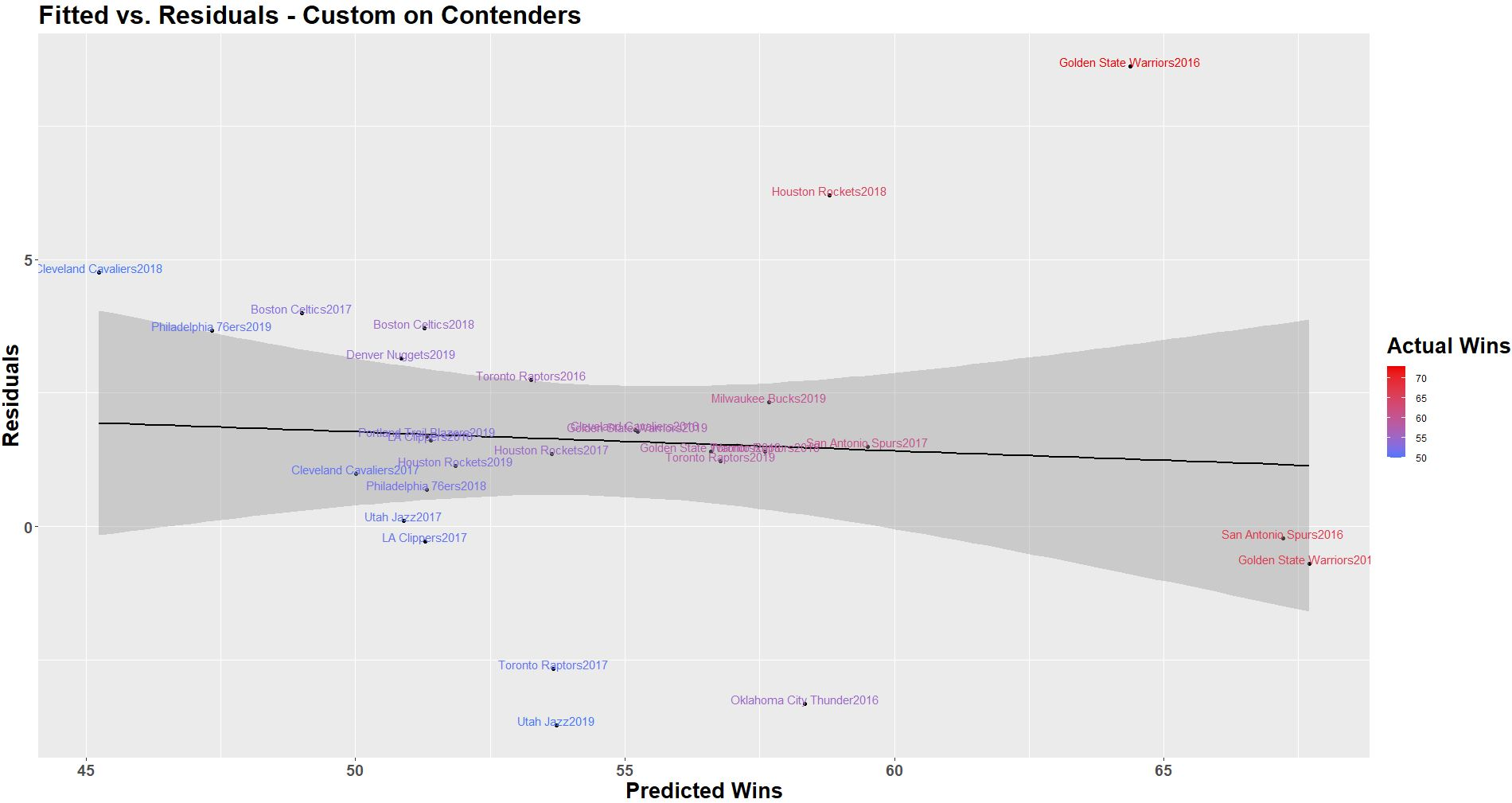
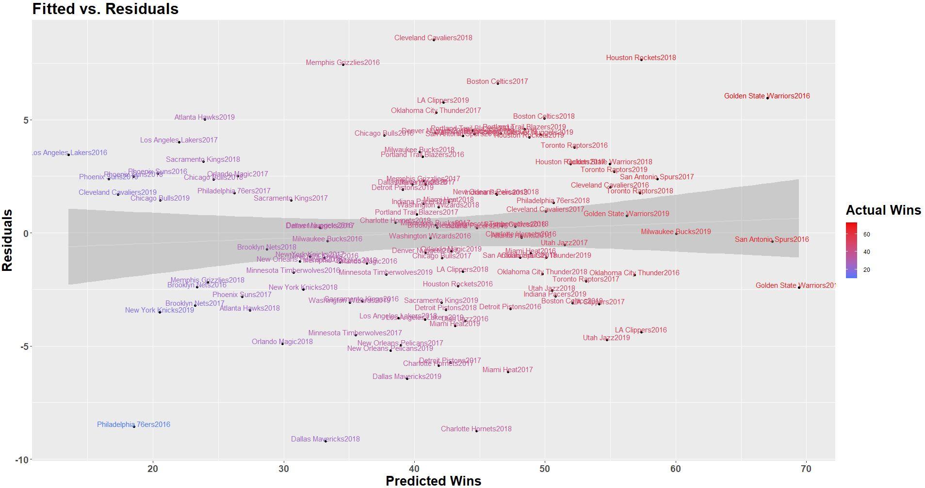
The predictions were plotted against the residuals to further understand the distribution of error among the data. With the Four Factors model, it seems as if the error is somewhat normally distributed, with the residual slightly increasing as team win totals increase, indicating the model is slightly weaker at predicting the win totals of the best teams in the league.
Though largely accurate, there is still room for improvement on the Four Factors model in terms of accuracy and the relevance of the information it communicates.
There is some divide among followers of the Four Factors with respect to their treatment of free throw rate. Traditionally, many people have used free throws attempted / field goals attempted as the free throw rate, however, this does not account for how accurate teams are at the free throw line, and simply states how often they get there. Using an alternative free throws made / field goals attempted would account for both frequency and accuracy of attempts. Despite this discrepancy in interpretation, and whichever side you fall on, I would still suggest incorporating both free throw rate (using FTA) and ft% as separate predictors such that you can understand how important each individual metric is in leading to wins, as each can be manipulated individually. One might question how a team can influence an opposing team’s ft%, and might claim that the only factor is the crowd (which is out of a team’s control), however, knowledge that a team has players that are weaker at free throws can alter the game plan to emphasize fouls against this player. The phrase “hack-a-shaq” was coined as this is a strategy that involves fouling a specific player (Shaquille O’Neal) due to his deficiency in shooting free throws. More recently, DeAndre Jordan (47.5% career FT shooter) has also suffered from this treatment. For a player who shoots roughly 50% from the line, he would average 1 point per possession per trip to the line. Compare this to a 2-point shot converting 50% of the time, or a 3-point shot converting 33% of the time, and you arrive at the same points per possession, however, when employed strategically, this tactic can “save” your team points. For example, shots in the paint and fast break opportunities are both highly efficient shot attempts (as they are converted more often), and thus, these situations are ideal for fouling your opponent (making it more difficult for them to earn the same number of points). This is the simplest mathematical justification for fouling, but there are several other considerations. The offensive rebounding rate after free throws for teams is closer to 10-12% Marc Jiang, which is much lower than the league average of 30%, and understandably so, as the offensive players are in a disadvantageous position to get the ball, so fouling makes it far more likely that the defense would secure possession of the ball after a shot. Repeatedly fouling a player inflicts physical and psychological damage to that player. Think back to “The Jordan Rules”, a strategy used to try to wear down Michael Jordan. Momentum and rhythm are at play as well. Slowing the pace of a game could adversely affect specific players and teams. A team can effectively prevent certain players from getting the same amount of touches that they would normally get by targeting their teammates, disrupting rhythm and slowing the momentum of a game. Though there is not data to strongly support this impact, people who have played basketball would agree that rhythm and momentum are important aspects of the game, and as such, strategies to create/disrupt rhythm and momentum are often encouraged. One of the main reasons for calling a time-out is to stop the momentum of a team on a run. People will often use the phrase that a player is “getting comfortable”, or "heating up" after hitting a few easy buckets. On the contrary, a player who is missing free throws can both negatively impact his own rhythm as well as his teammates' as they are not touching the ball as often. This impact, though more nuanced, illustrates one of the shortcomings of relying exclusively on numbers, as some aspects of the game cannot accurately be quantified at this point in time. Furthermore, given that ft% is a metric that certainly influences game plans (for the reasons above), it warrants its own value in the model that is separate from free throws attempted, as both are important to understand as standalone metrics.
Effective field goal% incorporates both 2-point and 3-point field goal attempts in order to give a single, cumulative metric, however, it is somewhat ambiguous. For example, a team that shoots 6-10 on 2-point attempts, and shoots no 3-point attempts, has an eFG% of 60%. Likewise, a team that shoots 3-8 on 2-point attempts and 2-2 on 3-point attempts also has a 60% eFG%. This is not sufficient for a coach, as their goal is to determine in which areas the team can improve, and to make actionable changes to make that improvement. It is imperative to understand efficiency by shot type such that the coach can hone in on a specific aspect of the offense (or defense). As currently constructed, this metric does not communicate the level of detail necessary to make these conclusions.
Again, the idea is to understand the efficiency of each shot type. Incorporating metrics such as 2-point FGA and 3-point FGA is problematic, though, as pace will influence these values (faster teams will shoot more shots). Also, simply taking field goal% for each shot type does not communicate the volume of shots by shot type. Instead, we should look at each on a relative basis (as a % of total field goal attempts). Additionally, we must consider accuracy and points awarded by each shot (2 vs. 3-point attempts). Collectively, these components can be combined to create a variable I will call weightedpointspershot.
Weight2ptshot <- 2pt attempts / Total FG Attempts
Weight3ptshot <- 3pt attempts / Total FG Attempts
Pointsper2ptA <- (2pt FG% * 2)
Pointsper3ptA <- (3pt FG% * 3)
Weightedpointsper2ptA <- Weight2ptshot * Pointsper2ptA
Weightedpointsper3ptA <- Weight3ptshot * Pointsper3ptA
The weightedpointspershotattempt can be added together to arrive at a metric commonly known as points per shot, but for practical takeaways, a coach should understand their efficiency by shot type in addition to a cumulative value.
Let me illustrate this feature through the following example.
A team attempts 600 2-point shots and 400 3-point shots. The team shoots 50% on 2-point attempts and 33% on 3-point attempts.
- Weight2ptshot <- (600 / 1000) = .6
- Weight3ptshot <- (400 / 1000) = .4
- Pointsper2ptA <- (.5 * 2) = 1
- Pointsper3ptA <- (.33 * 3) = 1
- Weightedpointsper2ptA <- (.6 * 1) = .6
- Weightedpointsper3ptA <- (.4 * 1) = .4
- Pointspershot <- (.6 + .4) = 1
The Houston Rockets in 2019 had the highest weightedpointsper3ptA of .55.
- % of shot attempts that are 3s = 51.9%
- 3-point made % = 35.6%
- weightedpointsper3ptA = (.519) * (.356 * 3) = .554292
The teams with the highest weightedpointsper3ptA:
- Houston Rockets2019
- Houston Rockets2018
- Houston Rockets2017
- Cleveland Cavaliers2017
- Golden State Warriors2016
It is no surprise that the Cavs and Warriors were in the championship in 2016 and 2017, and Houston had strong regular-season performances before getting nearly edged out by the Warriors (eventual champion/runner up each year from 2015-2019) in the playoffs. The leaders of this metric have been among the best in the league over the last few years.
To incorporate these features into the model, we need to do a bit of feature engineering. Using the other variables within the data (total FGA and 3-point FGA, we were able to find 2-point FGA and %). The weights (shot attempts by type as a % of total shot attempts) already existed, so we just needed to calculate the point per shot by multiplying the FG% by shot type with their points awarded (2 or 3). The same was done for opponents.
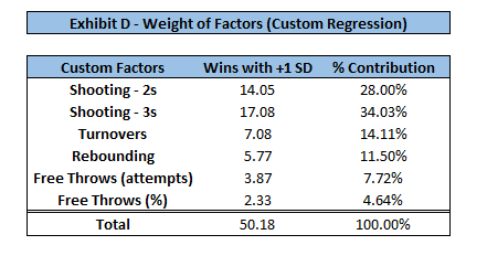
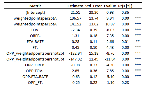
The additional variables were incorporated into the model (ft% and weighted points per 2-point and 3-point attempt) and the output is as follows:
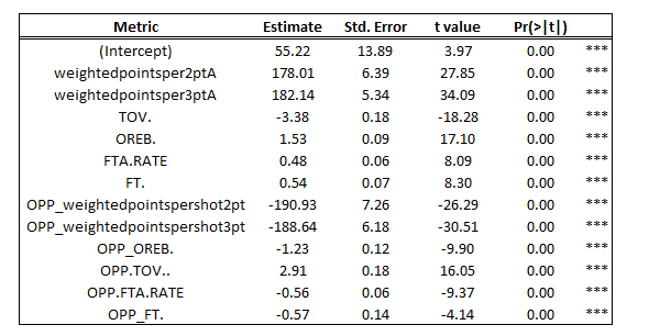
- Adjusted R2 = .94
- Standard Error = 3.01 (wins)
The custom model had higher accuracy on the testing set and recorded the following output:
- R2 = 0.94
- RMSE = 3.04
- 3.04 / 41 (Mean # of wins) = 7.41%
On average, the predictions were off 3.04 wins (7.41%), indicating that the model was slightly stronger (previously 8.66% error) in explaining the relationship between the variables than the traditional four factors.
 Values are rounded so calculations may be off
A team that is .25 standard deviations above average in weightedpointsper3ptA (value of .258 as opposed to .244) will win 2.63 more games. For a team that is .5 standard deviations above average in offensive rebounding, they will win 1.83 more games. A team that has both of these strengths will win 4.46 more games than league average. In reality, these values will not be so rounded, and a team might be .27 standard deviations above average in one metric, and .18 standard deviations below average in another metric.
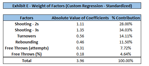
With the additional variables added to the model, the weights have shifted as well. Keep in mind, these factors reflect the sum of the offensive and defensive components. Once again, shooting is the most important factor of the game. The ability to shoot (and defend) 3-point shots is the most crucial factor in the model, followed by that of 2-point shots. The weights of the other factors have been shifted a bit, most notably turnovers losing much of their weight (previously 24.36% in Four Factor model). The coefficient is much larger on the weightedpointspershot variables as they are mostly values between 0 and 1, whereas all other metrics are between 0 and 100. Standardizing these variables did not change their weights/importance (exhibits D and E confirm this). Therefore, for ease of interpretation, I chose to leave the features on their original scale.
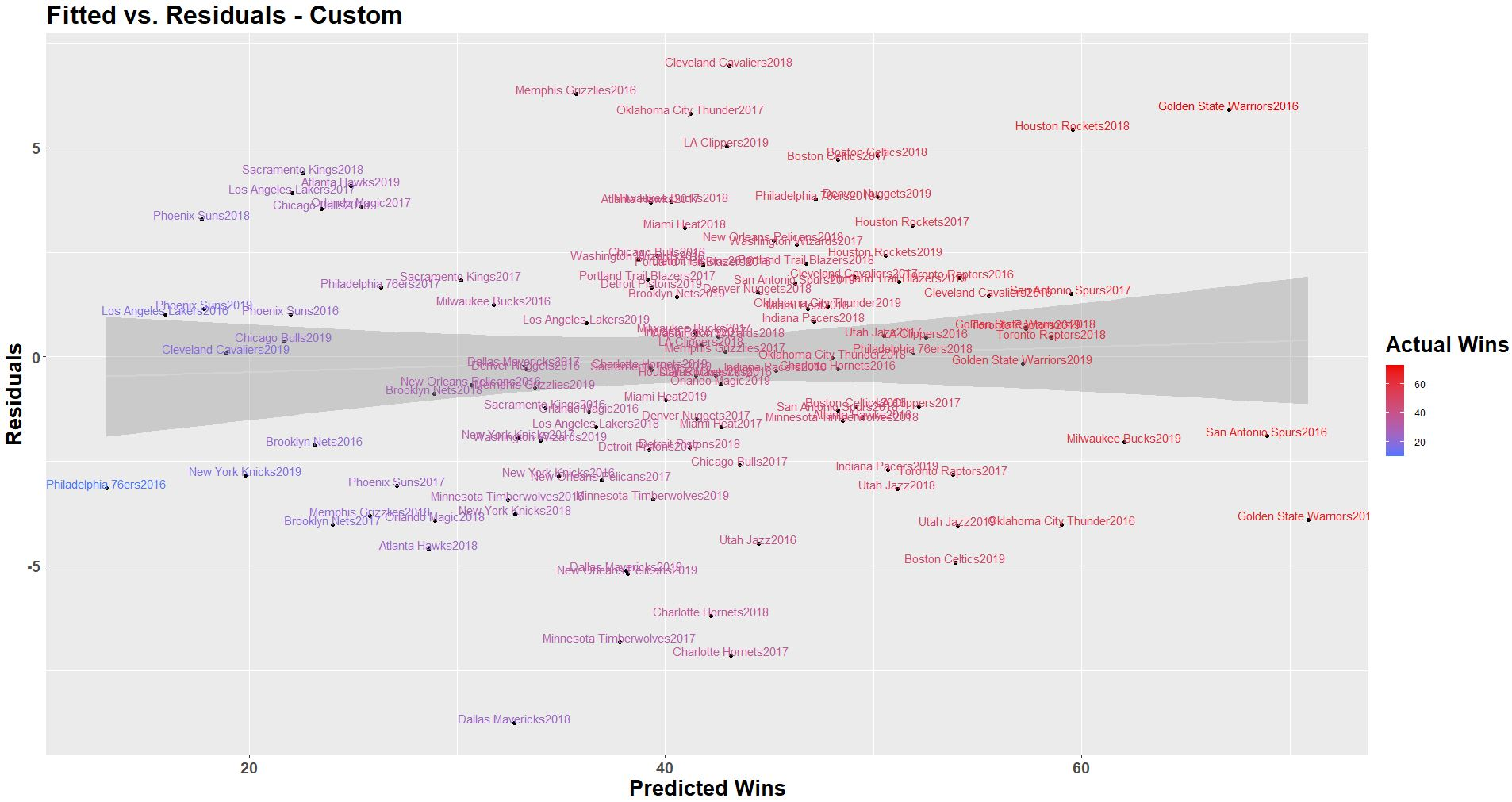
The output seems similar with the error appearing to be somewhat normally distributed.
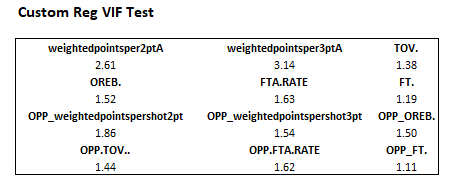
Some may raise the question of how incorporating the relative amount of shots by shot type as components of the weightedpointsperattempt influences correlation, so a VIF test was performed, and it indicated that multicollinearity is not high. If not satisfied with this approach, one might be able to train a model to communicate the same information by incorporating other variables, but it would result in a model that is more extensive than necessary. Overall, the custom model is more concise and less correlated than possible alternatives.
Though interesting to see how the model performs on all of the NBA teams, a more valuable analysis is to understand how it performs on championship contenders. For example, if a team is going to win 25 or 30 games, it is less important to understand exactly where in this range they will finish, as in the end, they are not playoff teams. For this reason, I wanted to test how well the model performs at predicting the win totals of top performing teams, as that will provide insight such as what “stats” make up a strong championship contender, and subsequently what roster decisions should be made to achieve those desired stats. To restrict the data to championship contenders, I searched the win totals of teams who have made the finals in recent years. Since 2005, 50 wins is the minimum number of regular-season wins of any team to make the finals, so we will use this as the minimum threshold for testing. That way, we are using our model to assess teams reasonably contending for an NBA championship. The resulting training set was comprised of 88 teams (who won at least 50 games between 2005 and 2015), and the testing set included 28 teams who won at least 50 games since 2016.
- Adjusted R-Squared = .62
- Standard Error = 2.83 (wins)
The results for the predictions were:
R-Squared = .66 RMSE = 3.37 games/56 (mean # of wins for teams above 50 wins) = 6.02%
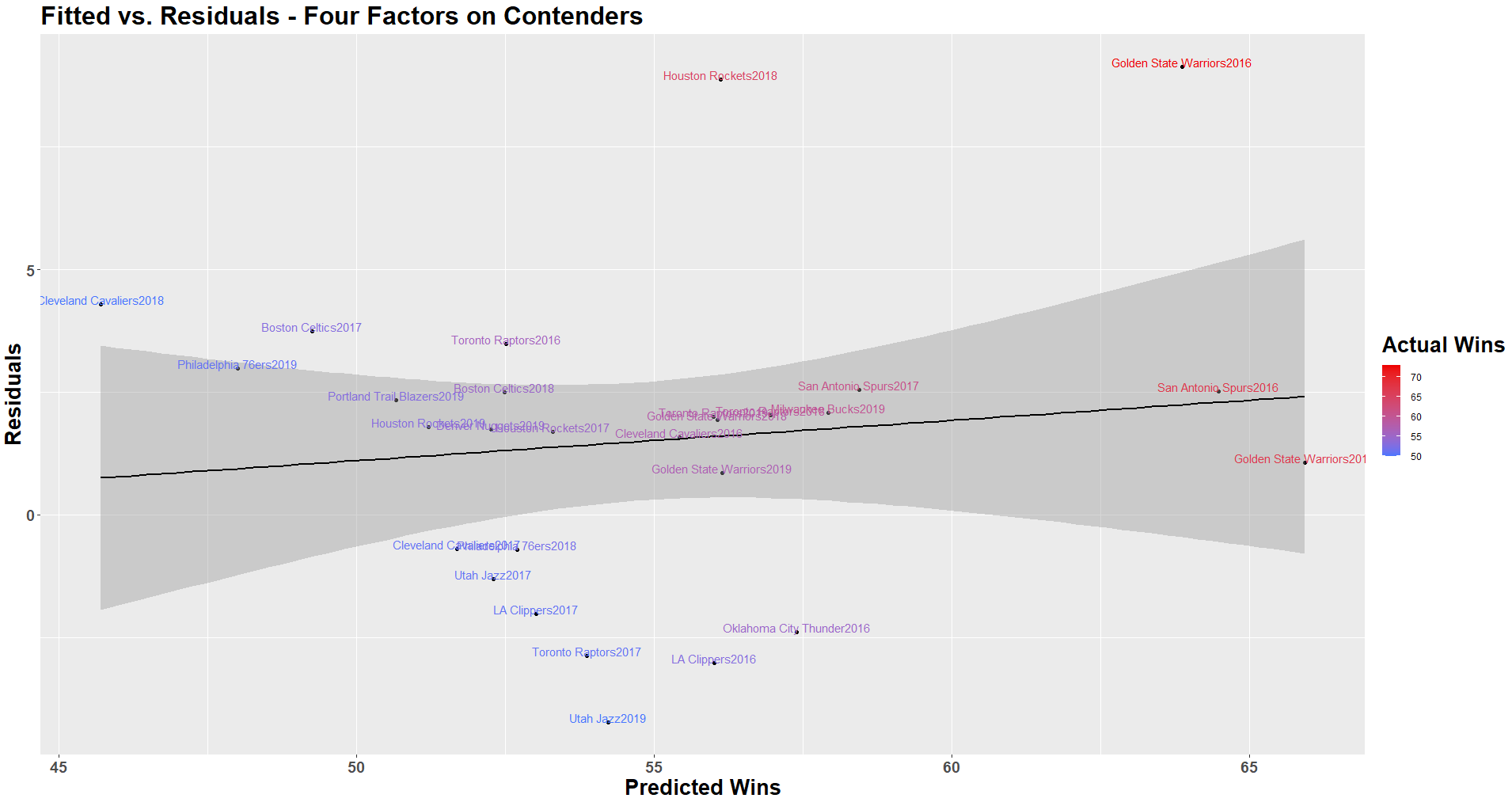
Again, residual value slightly increases with win total, indicating error increases for teams at the top of the league.
- Adjusted R-Squared = .70
- Standard Error = 2.54 (wins)
The custom model has lower error and a higher adjusted R-squared than the four factor model.
Results for predictions were:
- R-Squared = .72
- RMSE = 3.04 games/56 = 5.43%
Note here that the slight decrease in the trend line indicating the model is slightly stronger at predicting the top teams (lower residual error as wins increases). The model correctly predicted the number of wins for the SA Spurs of 2016, and was within one game of the GS Warriors of 2017 (both had 67 wins). Even with the 2016 GS Warriors positively skewing the error at the top of the league, the model performed strongly otherwise. While some may consider this GSW team of 2016 an outlier through “normal statistical tests”, in the context of this problem, I believe it is necessary to keep them in the data. Their season, though impressive, is repeatable under normal conditions, so it should be considered along with each other team. They may have some strength that is not highlighted in the model which is explaining their dominance (which warrants further investigation). Note that the R-squared values were lower for both regressions when used on contenders. This indicates there must be additional variables which may help explain the variation in performance among these teams (call to action for the community to do more work here).
Let’s recap. There were 2 main objectives in this analysis.
- Revisit Oliver’s Four Factor model to see if it is an accurate predictor in today’s NBA
- See if we can build a model that is more accurate and/or more insightful for teams
I concluded that Oliver's ranking of factors (shooting, turnovers, rebounding, free throws) was correct, but the weights of the factors should be slightly shifted (move some weight out of rebounding and free throws into shooting). In introducing a model that incorporated free throw% as well as weightedpointspershotattempt by shot type, we were able to build a model with that was a stronger predictor (albeit only half a game at the league-wide level), but more importantly, one that is more detailed, which communicates more useful information as to what areas for improvement exist for the team. Not only was the model more accurate on the aggregate of the entire league, but it was also more accurate for championship contenders, indicating it can better assess who will be truly competitive at the end of the year. By segmenting effective field goal% into a 2-point and 3-point metric, coaches can better understand how well their team is shooting and defending each shot type (in concise metrics that are still pace adjusted). They can act accordingly by changing the schematic approach to the game, or by rebuilding the roster accordingly. This finding is likely what has influenced the recent emphasis of the “3 and D” player, someone who excels at 3-point shooting and defense given their length/athleticism. At times, teams like the warriors and rockets have fully embraced this approach, starting 0 “true centers” and employing a lineup of a point guard + multiple players who are athletic and can shoot 3s, and it is no surprise to see them at the top of the league for the past few years.
Over time, as we saw with Oliver’s Four Factor model, it is likely that we see the weights of these factors shift with the meta of the NBA. Though the numbers suggest that certain factors are more important, it would be interesting to see if a team can go against the grain and be dominant, as styles still make fights. Can someone like Shaquille O’Neal (true center who scores primarily in the paint, lacks a jump shot and the lateral quickness to play on the perimeter) be as effective in today’s NBA? Some think not, but it would be interesting to see nevertheless. We have seen players who have flashed similar ability (Orlando Dwight Howard) who displayed a brief period of dominance despite not having a developed offensive skillset (poor touch around the rim, undeveloped counter moves and limited as a shooter). Had he been a more polished offensive player, or if there was a more recent example of a player with his physical gifts, they would likely pose a challenge to today’s style of play. Ideally, a player would be strong in each facet of the game, but reality is far from ideal. Some modern big guys are well rounded and have found much success in the league (Anthony Davis, Nikola Jokic, Joel Embiid), but these players are truly exceptional. Most big guys are either primarily shooters, or primarily back to the basket players. With the shift in emphasis on shooting and perimeter defending (as the data encourages), we are seeing the phasing out of back to the basket play, or situational use based on matchup. This presents a call to action to coaches from the youth level through college to continue to develop footwork and post moves in addition to just stressing shooting. Otherwise, we may never see if a contrasting style can challenge the current mold. We might be handicapping the next Shaquille O’Neal because he is spending too much time working on jump shots and not enough time on other fundamentals. This is just an example of how the meta of the game has influenced one position. Will we see other player types emerge in the coming years?
I explored the efficiency of 2-point and 3-point shot types, but 2-point shots can be further analyzed. Specifically, you can determine the efficiency of shots in the paint vs. mid-range shots to have even more granular information. The data I found showed how much scoring occurs in the paint vs. mid-range, but it did not list the shot attempts for each area, so I could not determine how efficient each team was in the paint and from mid-range. There was a negative correlation between wins and % of points scored from mid-range, which indicates that better teams are not utilizing this area of the floor as much (as expected), but it might still be worthwhile to explore. Recording play-by-play information to evaluate statistics by play-call and situation (“isolation”, “pick-and-roll”), or even the side of the floor would be immensely valuable. The insight from these can help pinpoint the strengths/weaknesses of players in a way that aggregate statistics do not. This would require extensive film study and basketball knowledge, but would likely be worthwhile in the long-run.