AI Art with Deep Learning

A walkthrough of three models that paint, translate, and reimagine images — Neural Style Transfer, Pix2Pix, and CycleGAN.

Table of Contents

• Motivation
• Neural Style Transfer
  • Content Cost
  • Style Cost
  • Total Variation (TV) Cost
  • Experiments
  • Results
  • Where it went from here
• Pix2Pix
  • Loss Function
  • Network Architecture
  • Training Details
  • Results
  • Where it went from here
• CycleGAN
  • Motivation
  • Loss Formulation
  • Key Takeaways
  • Network Architecture
  • Results
  • Where it went from here
• Closing thoughts
• Updates

---

Motivation

Creativity is something we closely associate with what it means to be human. But with digital technology now enabling machines to recognize, learn from, and respond to humans, an inevitable question follows: Can machines be creative?

It could be argued that the ability of machines to learn what things look like, and then make convincing new examples marks the advent of creative AI. This tutorial will cover three different Deep Learning models to create novel arts, solely by code — Neural Style Transfer, Pix2Pix, and CycleGAN. They build on each other in a natural way: NST optimizes a single image against a pretrained network without any training of its own, Pix2Pix learns a paired mapping with a conditional GAN, and CycleGAN drops the paired-data requirement entirely.

---

Neural Style Transfer

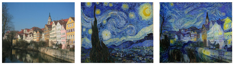
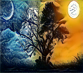
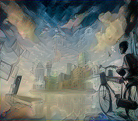
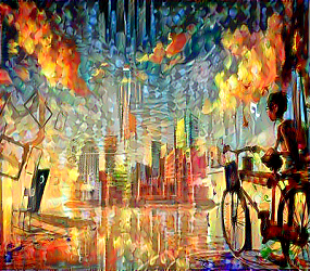
Style Transfer is one of the most fun techniques in Deep learning. It combines two images, namely, a Content image (C) and a Style image (S), to create an Output image (G). The Output image has the content of image C painted in the style of image S.

Style Transfer uses a pre-trained Convolutional Neural Network to get the content and style representations of the image, but why do these intermediate outputs within the pre-trained image classification network allow us to define style and content representations?

A network trained on image classification has learned to convert raw pixels into a progressively richer internal representation of what's in the image. The activation maps of the first few layers represent low-level features like edges and textures; as we go deeper through the network, the activation maps represent higher-level features — objects like wheels, or eyes, or faces. Style Transfer incorporates three different kinds of losses:

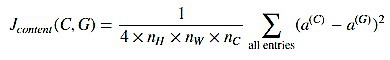
• Content Cost: $J_{\text{Content}}(C, G)$
• Style Cost: $J_{\text{Style}}(S, G)$
• Total Variation (TV) Cost: $J_{\text{TV}}(G)$

Putting it all together:

$$J_{\text{Total}}(G) = \alpha \cdot J_{\text{Content}}(C, G) + \beta \cdot J_{\text{Style}}(S, G) + \gamma \cdot J_{\text{TV}}(G)$$

Let's delve deeper to know more profoundly what's going on under the hood!

Content Cost

Usually, each layer in the network defines a non-linear filter bank whose complexity increases with the position of the layer in the network. Content loss tries to make sure that the Output image G has similar content as the Input image C, by minimizing the L2 distance between their activation maps.

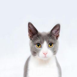
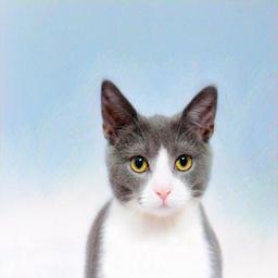
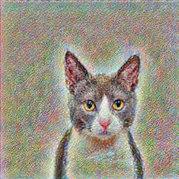
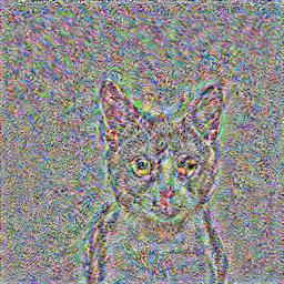
Practically, we get the most visually pleasing results if we choose a layer in the middle of the network — neither too shallow nor too deep. The higher layers in the network capture the high-level content in terms of objects and their arrangement in the input image but do not constrain the exact pixel values of the reconstruction very much. In contrast, reconstructions from the lower layers simply reproduce the exact pixel values of the original image.

Let $a(C)$ be the hidden layer activations which is a $N_h \times N_w \times N_c$ dimensional tensor, and let $a(G)$ be the corresponding hidden layer activations of the Output image. Finally, the Content Cost function is defined as follows:

$N_h$, $N_w$, $N_c$ are the height, width, and the number of channels of the hidden layer chosen. To compute the cost $J_{\text{Content}}(C, G)$, it might also be convenient to unroll these 3D volumes into a 2D matrix, as shown below.

The first image is the original one, while the remaining ones are the reconstructions when layers Conv_1_2, Conv_2_2, Conv_3_2, Conv_4_2, and Conv_5_2 (left to right and top to bottom) are chosen in the Content loss.

Style Cost

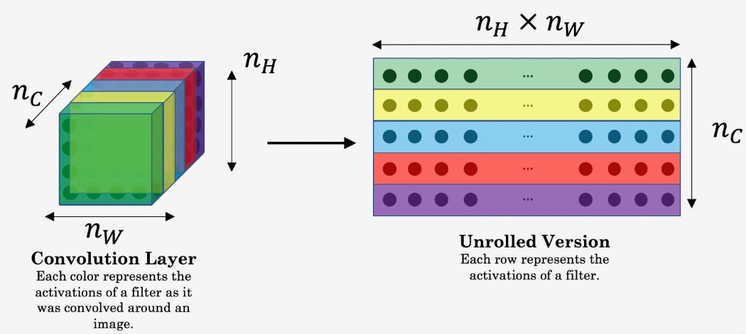
To understand it better, we first need to know something about the Gram Matrix. In linear algebra, the Gram matrix $G$ of a set of vectors $(v_1, \ldots, v_n)$ is the matrix of dot products, whose entries are $G(i, j) = v_i^\top v_j$. In other words, $G(i, j)$ compares how similar $v_i$ is to $v_j$. If they are highly similar, the outcome would be a large value, otherwise it would be low, suggesting a lower correlation. In Style Transfer, we can compute the Gram matrix by multiplying the unrolled filter matrix with its transpose as shown below:

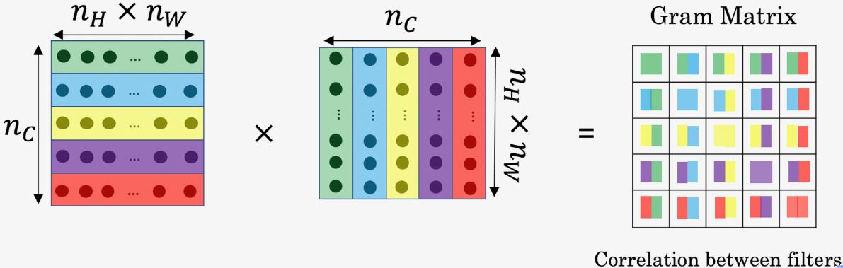
The result is a matrix of dimension $(n_C, n_C)$ where $n_C$ is the number of filters. The value $G(i, j)$ measures how similar the activations of filter $i$ are to the activations of filter $j$. One important part of the gram matrix is that the diagonal elements such as $G(i, i)$ measure how active filter $i$ is. For example, suppose filter $i$ is detecting vertical textures in the image, then $G(i, i)$ measures how common vertical textures are in the image as a whole.

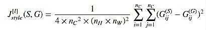
By capturing the prevalence of different types of features $G(i, i)$, as well as how much different features occur together $G(i, j)$, the Gram matrix $G$ measures the Style of an image. Once we have the Gram matrix, we minimize the L2 distance between the Gram matrix of the Style image S and the Output image G. Usually, we take more than one layer into account to calculate the Style cost as opposed to Content cost (which only requires one layer), and the reason for doing so is discussed later on in the post. For a single hidden layer, the corresponding style cost is defined as:

Total Variation (TV) Cost

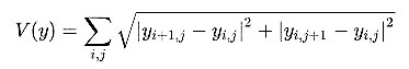
It acts like a regularizer that encourages spatial smoothness in the generated image (G). This was not used in the original paper proposed by Gatys et al., but it sometimes improves the results. For a 2D signal (or image), it is defined as follows:

Experiments

What happens if we zero out the coefficients of the Content and TV loss, and consider only a single layer to compute the Style cost?

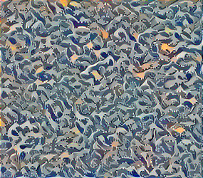
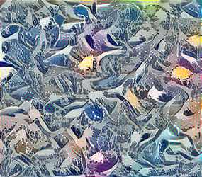
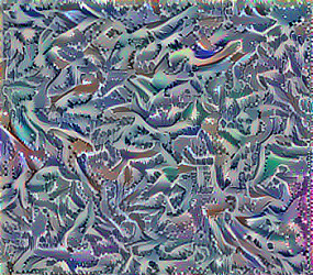
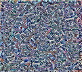
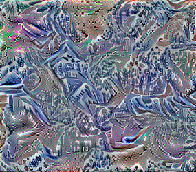
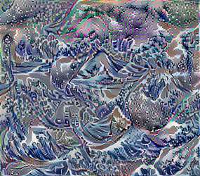
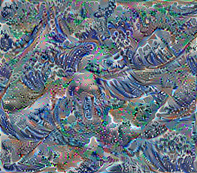
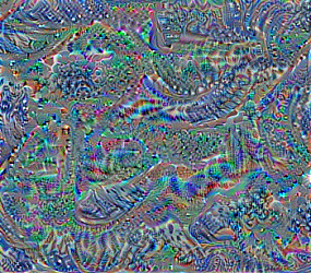
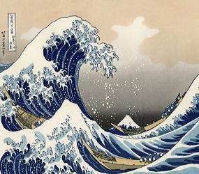
As many of you might have guessed, the optimization algorithm will now only minimize the Style cost. So, for a given Style image, we will see the different kinds of brush-strokes (depending on the layer used) that the model will try to enforce in the final generated image (G). Remember, we started with a single layer in the Style cost, so running the experiments for different layers would give different kinds of brush-strokes. Suppose the style image is the famous The Great Wave off Kanagawa shown below:

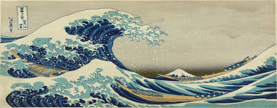
The brush-strokes that we get after running the experiment, taking different layers one at a time, are attached below.

These are brush-strokes that the model learned when layers Conv_2_2, Conv_3_1, Conv_3_2, Conv_3_3, Conv_4_1, Conv_4_3, Conv_4_4, Conv_5_1, and Conv_5_4 (left to right and top to bottom) were used one at a time in the Style cost.

The reason behind running this experiment was that the authors of the original paper gave equal weightage to the styles learned by different layers while calculating the Total Style Cost. Now, that's not intuitive at all after looking at these images, because we can see that styles learned by the shallower layers are much more aesthetically pleasing compared to what deeper layers learned. So, we would like to assign a lower weight to the deeper layers and higher to the shallower ones (exponentially decreasing the weightage could be one way).

Results

Where it went from here

The original Gatys et al. approach was slow — each new output image required hundreds of optimization steps against a frozen VGG. The follow-up literature has largely been about making it faster and then making it work for arbitrary styles at test time. Two papers capture that arc cleanly:

No code or results for either of these in this post — the writeups below are just for reference.

Perceptual Losses for Real-Time Style Transfer and Super-Resolution — Johnson, Alahi, Fei-Fei (2016)

The key move: instead of optimizing one image at a time, train a separate feed-forward network to do the stylization in a single pass. The training objective is the same perceptual loss as Gatys et al. — feature reconstruction against a pretrained VGG (content) plus Gram-matrix matching across multiple VGG layers (style) — but the loss now serves as a target for a network being trained on a large image dataset, rather than as an objective for per-image optimization.

At test time, stylizing a new image is just one forward pass through the trained transformation network — orders of magnitude faster than Gatys et al. The trade-off is that you now have to train a separate network for every style: the model is locked to whatever style image was used during training. Quality is broadly comparable to optimization-based NST, slightly worse in some cases, but in exchange you get real-time inference.

Arbitrary Style Transfer with Adaptive Instance Normalization — Huang & Belongie (2017)

This paper drops the "one network per style" constraint entirely. The key observation: Instance Normalization (which had been observed to work better than batch norm for style transfer networks) can be reinterpreted as performing a kind of style normalization — it removes per-instance style information by normalizing the mean and variance of feature maps. So if you make the normalization adaptive — feeding in the desired mean and variance from a style image rather than learning them — you can transfer arbitrary styles at test time.

Concretely, AdaIN is defined as:

$$\text{AdaIN}(x, y) = \sigma(y) \cdot \left( \frac{x - \mu(x)}{\sigma(x)} \right) + \mu(y)$$

where $x$ is the content feature map, $y$ is the style feature map, and $\mu$ and $\sigma$ are channel-wise mean and standard deviation computed across spatial locations. Aligning the channel-wise mean and variance of $x$ to those of $y$ transfers the style.

The architecture is a VGG encoder (fixed, pretrained on ImageNet) plus a learned decoder that roughly mirrors the encoder. Content and style images both get encoded; AdaIN is applied at an intermediate VGG layer; the result is decoded back to image space. The decoder is trained with a content loss (against the AdaIN output) and a style loss (matching mean and standard deviation of decoder activations to those of the style image at multiple VGG layers).

The result is what most modern "real-time arbitrary style transfer" demos use: one trained model, any style image at test time, a single forward pass.

---

Pix2Pix

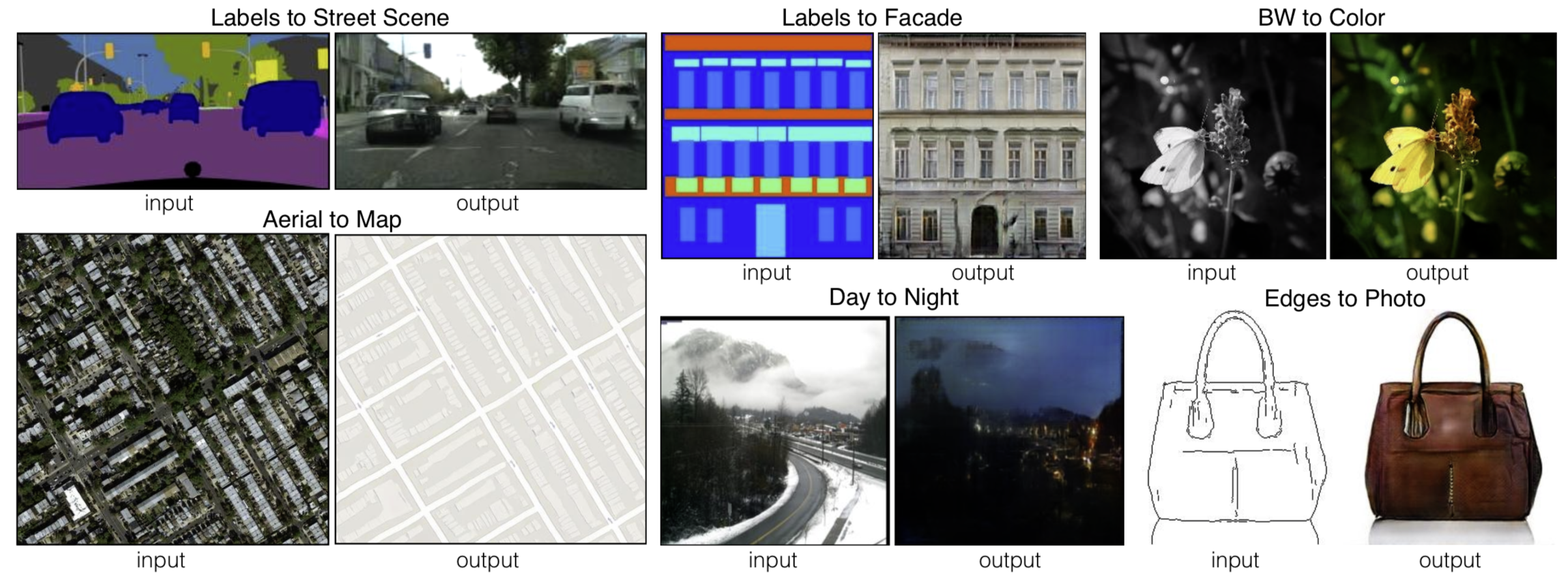
Image-to-image translation is the task of taking one representation of a scene — an edge map, a semantic label map, or a daytime photograph — and producing another representation of the same scene: a sketch turned into a colored photo, a label map turned into a street view, a daytime shot turned into night. Pix2Pix made this work across many such problems with a single recipe.

If you don't know what Generative Adversarial Networks are, please refer to this blog before going ahead; it explains the intuition and mathematics behind the GANs.

Authors of this paper investigated Conditional adversarial networks as a general-purpose solution to Image-to-Image Translation problems. These networks not only learn the mapping from the input image to the output image but also learn a loss function to train this mapping. If we take a naive approach and ask a CNN to minimize just the Euclidean distance between predicted and ground truth pixels, it tends to produce blurry results; minimizing Euclidean distance averages all plausible outputs, which causes blurring.

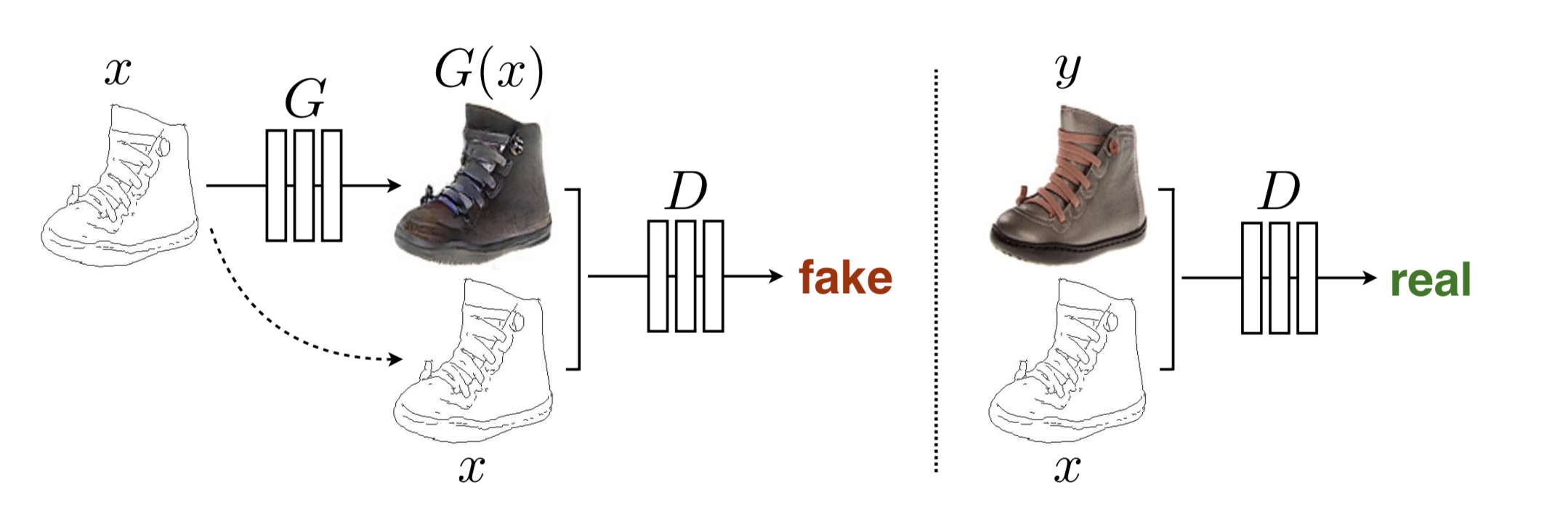
In Generative Adversarial Networks settings, we could specify only a high-level goal, like "make the output indistinguishable from reality", and then it automatically learns a loss function appropriate for satisfying this goal. The conditional generative adversarial network, or cGAN for short, is a type of GAN that involves the conditional generation of images by a generator model. Like other GANs, Conditional GAN has a discriminator (or critic depending on the loss function we are using) and a generator, and the overall goal is to learn a mapping, where we condition on an input image and generate a corresponding output image. In analogy to automatic language translation, automatic image-to-image translation is defined as the task of translating one possible representation of a scene into another, given sufficient training data.

Most formulations treat the output space as "unstructured" in the sense that each output pixel is considered conditionally independent from all others given the input image. Conditional GANs instead learn a structured loss. Structured losses penalize the joint configuration of the output. Mathematically, CGANs learn a mapping from observed image $x$ and random noise vector $z$, to $y$, i.e. $G: {x, z} \to y$. The generator $G$ is trained to produce output that cannot be distinguished from the real images by an adversarially trained discriminator, $D$, which in turn is optimized to perform best at identifying the fake images generated by the generator. The figure shown below illustrates the working of GAN in the Conditional setting.

Loss Function

The objective of a conditional GAN can be expressed as:

$$\mathcal{L}_{\text{cGAN}}(G, D) = \mathbb{E}_{x, y}[\log D(x, y)] + \mathbb{E}_{x, z}[\log (1 - D(x, G(x, z)))]$$

where $G$ tries to minimize this objective against an adversarial $D$ that tries to maximize it. It is beneficial to mix the GAN objective with a more traditional loss, such as L1 distance, to make sure that the ground truth and the output are close to each other in the L1 sense:

$$\mathcal{L}_{L1}(G) = \mathbb{E}_{x, y, z}\left[ | y - G(x, z) |_1 \right]$$

Without $z$, the net could still learn a mapping from $x$ to $y$, but would produce deterministic output, and therefore would fail to match any distribution other than a delta function. So, the authors provided noise in the form of dropout, applied on several layers of the generator at both training and test time. Despite the dropout noise, there is only minor stochasticity in the output. The complete objective is now:

$$G^* = \arg \min_G \max_D \mathcal{L}_{\text{cGAN}}(G, D) + \lambda \cdot \mathcal{L}_{L1}(G)$$

The Min-Max objective mentioned above was proposed by Ian Goodfellow in 2014 in his original paper, but unfortunately it doesn't perform well because of the vanishing gradients problem. Since then, there has been a lot of development, and many researchers have proposed different kinds of loss formulations (LS-GAN, WGAN, WGAN-GP) to alleviate vanishing gradients. Authors of this paper used the Least-square objective function while optimizing the networks, which can be expressed as:

$$\min_D \mathcal{L}_{\text{LSGAN}}(D) = \tfrac{1}{2} \mathbb{E}_{x, y}\left[(D(x, y) - 1)^2\right] + \tfrac{1}{2} \mathbb{E}_{x, z}\left[D(x, G(x, z))^2\right]$$

$$\min_G \mathcal{L}_{\text{LSGAN}}(G) = \tfrac{1}{2} \mathbb{E}_{x, z}\left[(D(x, G(x, z)) - 1)^2\right]$$

Network Architecture

Generator

Assumption: The input and output differ only in surface appearance and are renderings of the same underlying structure. Therefore, structure in the input is roughly aligned with the structure in the output. The generator architecture is designed around these considerations only. For many image translation problems, there is a great deal of low-level information shared between the input and output, and it would be desirable to shuttle this information directly across the net. To give the generator a means to circumvent the bottleneck for information like this, skip connections are added following the general shape of a U-Net.

Specifically, skip connections are added between each layer i and layer n − i, where n is the total number of layers. Each skip connection simply concatenates all channels at layer i with those at layer n − i. The U-Net encoder-decoder architecture is:

• Encoder: C64 - C128 - C256 - C512 - C512 - C512 - C512 - C512
• U-Net Decoder: C1024 - CD1024 - CD1024 - CD1024 - C512 - C256 - C128

where:

• Ck — a Convolution - BatchNorm - ReLU layer with k filters.
• CDk — a Convolution - BatchNorm - Dropout - ReLU layer with k filters and a dropout rate of 50%.

Discriminator

The GAN discriminator models the high-frequency structure term, and relies on the L1 term to force low-frequency correctness. To model high frequencies, it is sufficient to restrict the attention to the structure in local image patches. Therefore, the discriminator architecture was termed PatchGAN — it only penalizes structure at the scale of patches. This discriminator tries to classify whether each N × N patch in an image is real or fake. The discriminator is run convolutionally across the image, and the responses get averaged out to provide the ultimate output.

Patch GAN discriminators effectively model the image as a Markov random field, assuming independence between pixels separated by more than a patch diameter. The receptive field of the discriminator used was 70 × 70 and was performing best compared to other smaller and larger receptive fields.

• 70 × 70 PatchGAN: C64 - C128 - C256 - C512

The diagrams attached below show the forward and backward propagation through the generator and discriminator!

Training Details

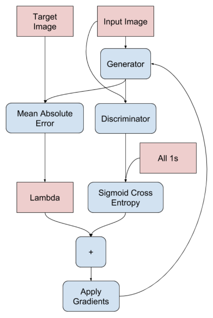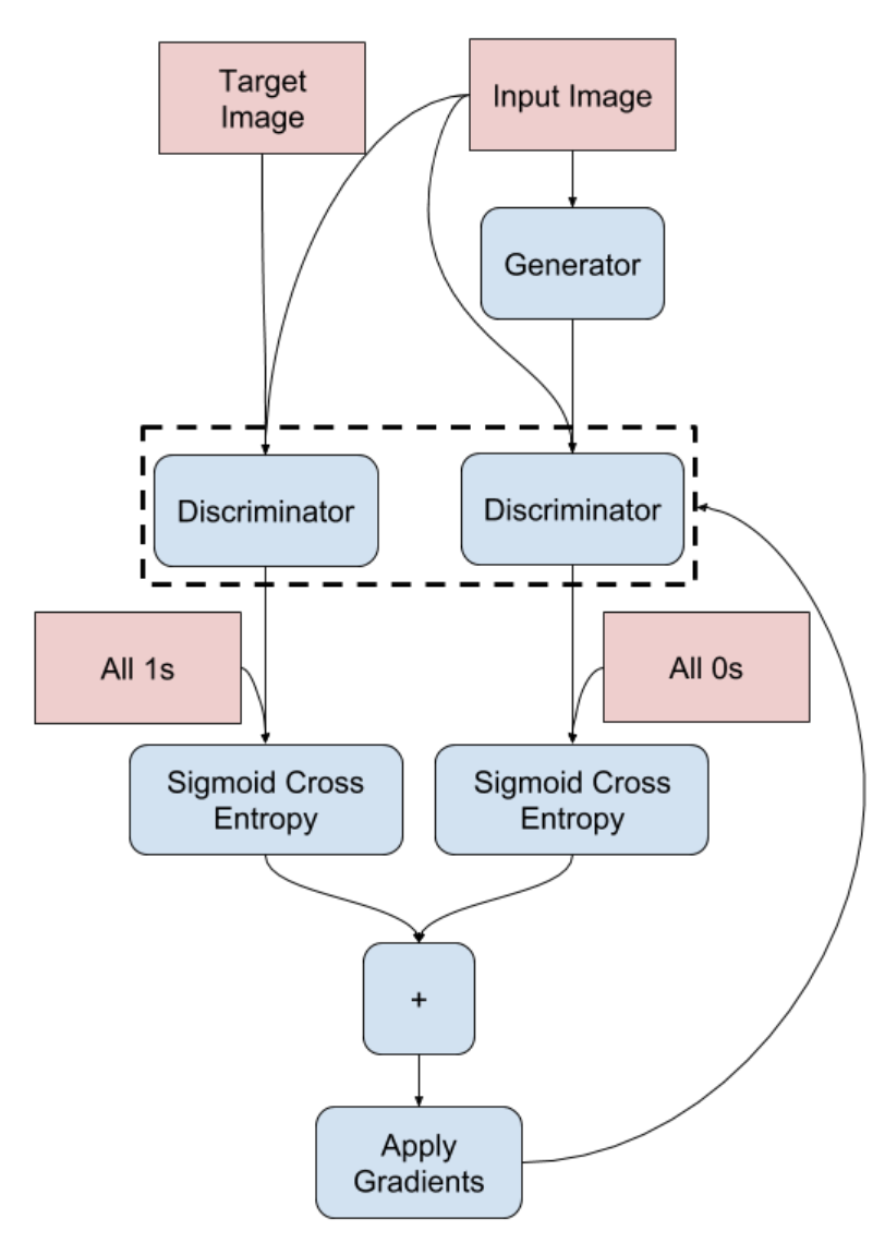• All convolution kernels are of size 4 × 4.
• Dropout is used both at training and test time.
• Instance normalization is used instead of batch normalization.
• Normalization is not applied to the first layer in the encoder and discriminator.
• Adam is used with a learning rate of 2e-4, with momentum parameters β1 = 0.5, β2 = 0.999.
• All ReLUs in the encoder and discriminator are leaky, with slope 0.2, while ReLUs in the decoder are not leaky.

Results

Cityscapes

Facades

Where it went from here

Pix2Pix worked beautifully at 256 × 256 but two limitations showed up quickly: it didn't scale cleanly to higher resolutions, and semantic-map conditioning was relatively coarse because the segmentation input got washed out by normalization layers in the generator. Two papers from the NVIDIA group addressed these directly:

No code or results for either of these in this post — the writeups below are just for reference.

Pix2PixHD — High-Resolution Image Synthesis and Semantic Manipulation with Conditional GANs — Wang et al. (2018)

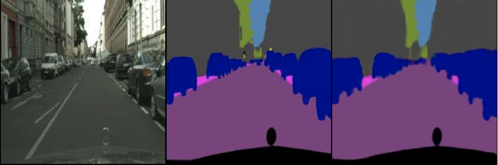
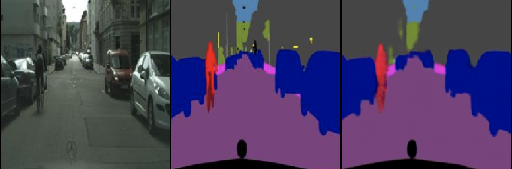
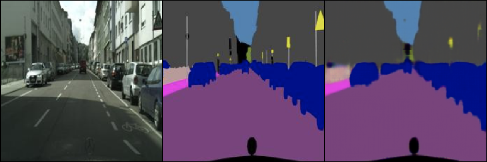
The headline result was producing 2048 × 1024 images conditioned on Cityscapes-style semantic label maps — an order of magnitude more pixels than Pix2Pix could comfortably handle. Three ingredients made this work:

• Coarse-to-fine generator. A global generator G1 first produces a 1024 × 512 image; then a local enhancer G2 takes both the input label map at full resolution and G1's output, and produces the final 2048 × 1024 image. The two networks are trained jointly after a brief warm-up of G1 alone. The split lets G1 focus on global structure while G2 sharpens local detail.
• Multi-scale discriminators. Three discriminators with the same PatchGAN architecture but operating at different image scales (the full-resolution image and downsampled versions). Each judges patches at its own scale — the coarser ones see more global structure, the finer one judges local realism.
• Feature-matching loss. A perceptual-style loss computed from the discriminators themselves: features extracted at multiple layers of the discriminators on the real image should match those on the generated image. This stabilizes training at high resolutions where the raw adversarial loss alone gets unstable.

Pix2PixHD also supported instance-level editing — feeding instance boundary maps in addition to semantic labels — which let users add, remove, or move individual objects in the synthesized scene.

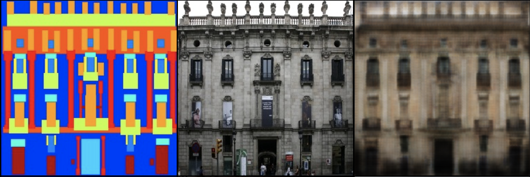
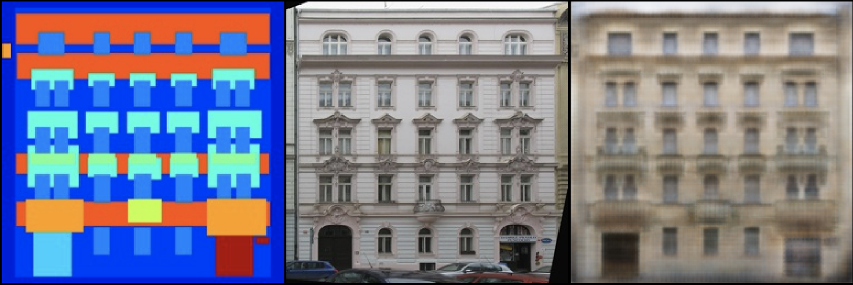
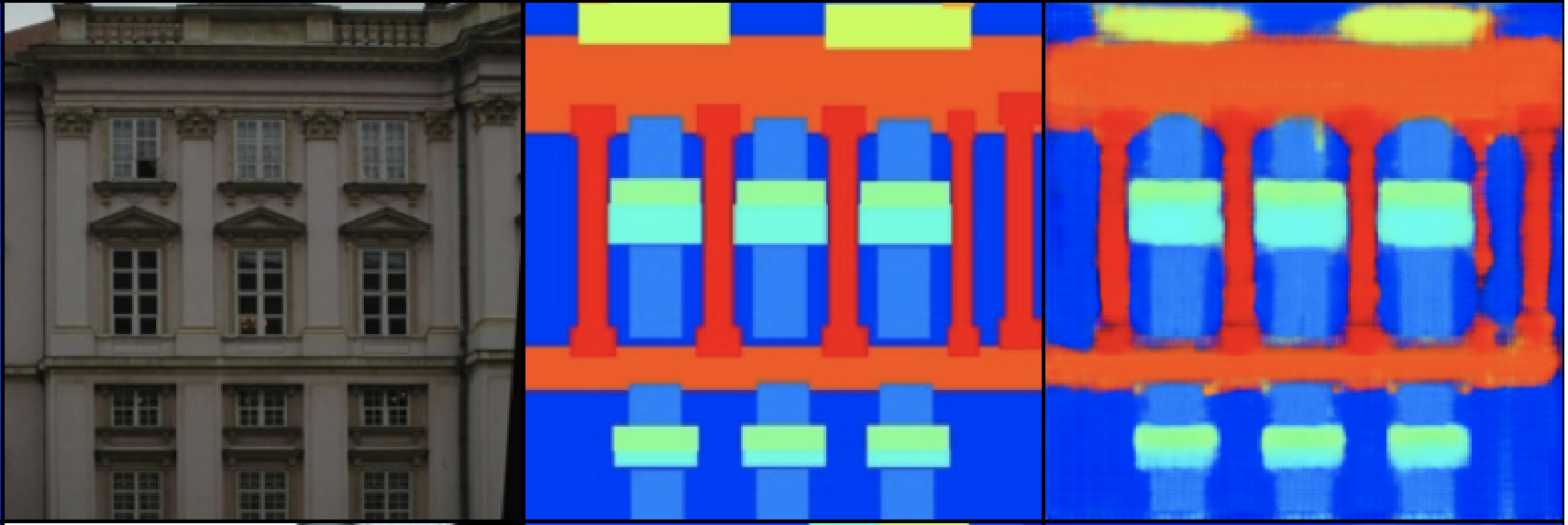
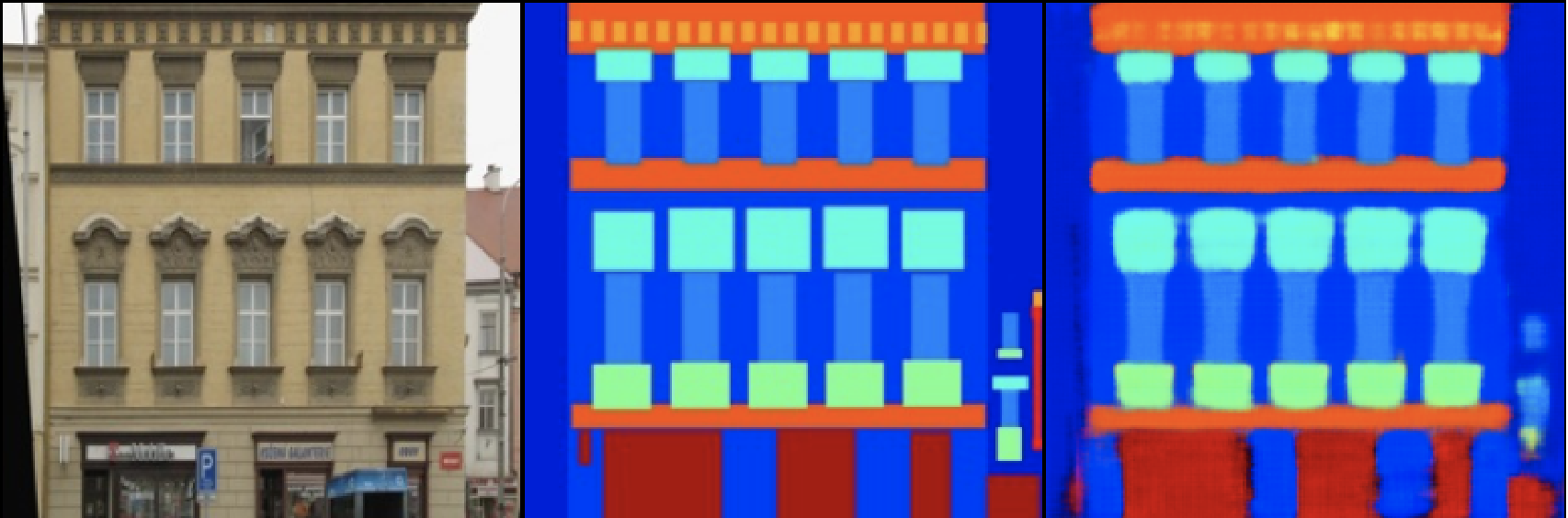
GauGAN / SPADE — Semantic Image Synthesis with Spatially-Adaptive Normalization — Park et al. (2019)

The diagnosis here was sharper. When you feed a semantic segmentation map only at the input of a generator, the information gets diluted by every batch-norm or instance-norm layer in the network: normalization subtracts a mean and divides by a standard deviation that's computed across spatial dimensions, which throws away exactly the spatial structure the segmentation map was supposed to provide.

The fix is the SPADE (Spatially-Adaptive Denormalization) block. After the normalization step, instead of applying a per-channel affine transform with learned scalar $\gamma$ and $\beta$, SPADE uses $\gamma$ and $\beta$ that are functions of the segmentation map, varying per spatial location:

$$\text{SPADE}(x, m)_{i, j, c} = \gamma_{c, i, j}(m) \cdot \left( \frac{x_{i, j, c} - \mu_c}{\sigma_c} \right) + \beta_{c, i, j}(m)$$

where $m$ is the segmentation map and $\gamma$, $\beta$ are produced by a small conv network that takes $m$ (appropriately downsampled) as input. Crucially, this is done at every normalization layer in the generator — so the segmentation map is re-injected at every resolution, never washed out.

SPADE was the engine behind NVIDIA's GauGAN demo (the "paint a landscape from a label map" tool) and produced visibly more faithful semantic synthesis than Pix2PixHD: regions stayed where you drew them, objects didn't bleed across boundaries, and texture varied correctly with the label class.

---

CycleGAN

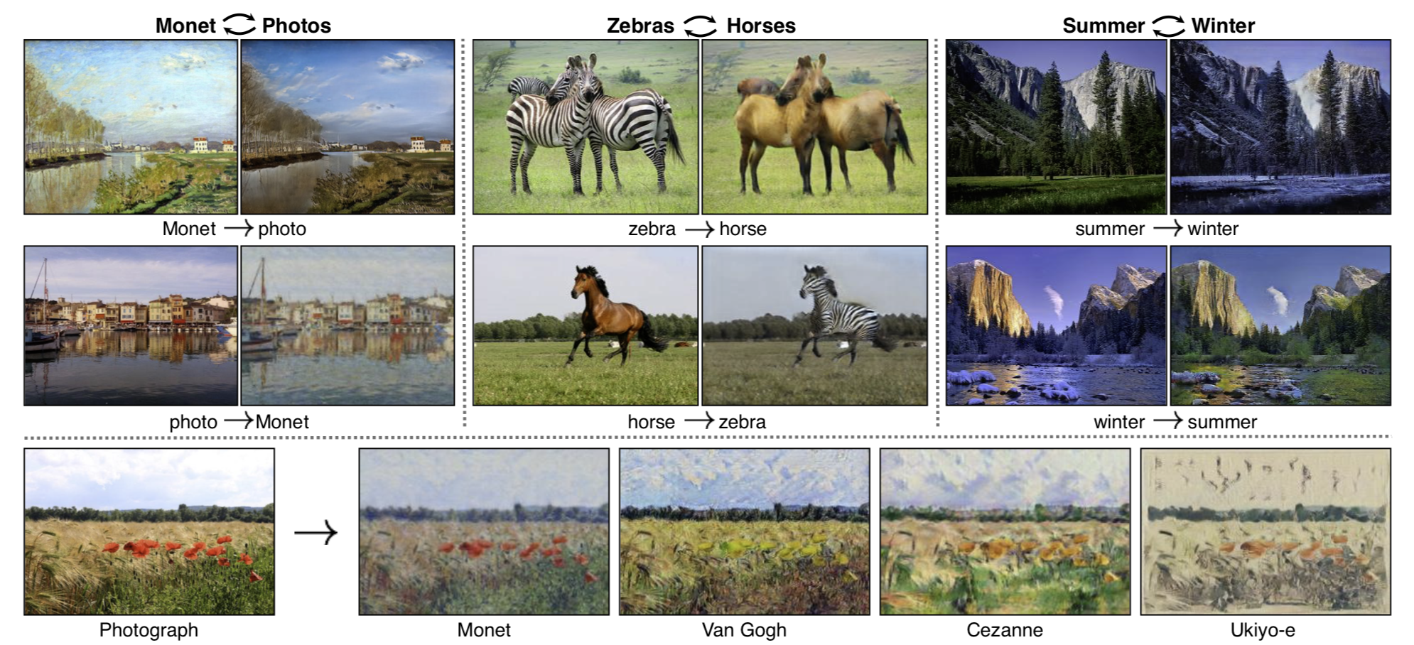
Pix2Pix needed paired data — for every input image, you needed a matching output image. CycleGAN drops that requirement. The image-to-image translation is a class of vision and graphics problems where the goal is to learn the mapping between an input image and an output image using a training set of aligned image pairs. However, for many tasks, paired training data is not available, so the authors of this paper presented an approach for learning to translate an image from a source domain $X$ to a target domain $Y$ in the absence of paired examples.

The goal is to learn a mapping $G: X \to Y$ such that the distribution of images $G(X)$ is indistinguishable from the distribution $Y$ using an adversarial loss. Because this mapping is highly under-constrained, they coupled it with an inverse mapping $F: Y \to X$ and introduced a cycle consistency loss to enforce $F(G(X)) \approx X$ (and vice-versa).

Motivation

Obtaining paired training data can be difficult and expensive. For example, only a couple of datasets exist for tasks like semantic segmentation, and they are relatively small. Obtaining input-output pairs for graphics tasks like artistic stylization can be even more difficult since the desired output is highly complex, and typically requires artistic authoring. For many tasks, like object transfiguration (e.g., zebra ↔ horse), the desired output is not even well-defined. Therefore, the authors tried to present an algorithm that can learn to translate between domains without paired input-output examples. The primary assumption is that there exists some underlying relationship between the domains.

Although there is a lack of supervision in the form of paired examples, supervision at the level of sets can still be exploited: one set of images in domain $X$ and a different set in domain $Y$. The optimal $G$ thereby translates the domain $X$ to a domain $\hat{Y}$ distributed identically to $Y$. However, such a translation does not guarantee that an individual input $x$ and output $y$ are paired up in a meaningful way — there are infinitely many mappings $G$ that will induce the same distribution over $y$.

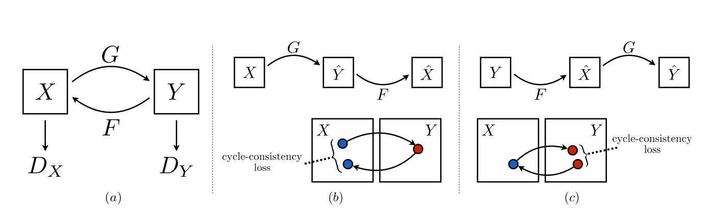
As illustrated in the figure, the model includes two mappings $G: X \to Y$ and $F: Y \to X$. Besides, two adversarial discriminators are introduced, $D_X$ and $D_Y$; the task of $D_X$ is to discriminate images $x$ from translated images $F(y)$, whereas $D_Y$ aims to discriminate $y$ from $G(x)$. So, the final objective has two different loss terms: adversarial loss for matching the distribution of generated images to the data distribution in the target domain, and cycle consistency loss to prevent the learned mappings $G$ and $F$ from contradicting each other.

Loss Formulation

Adversarial Loss

Adversarial loss is applied to both the mapping functions — $G: X \to Y$ and $F: Y \to X$. $G$ tries to generate images $G(x)$ that look similar to images from domain $Y$, and $D_Y$ tries to distinguish the translated samples $G(x)$ from real samples $y$ (a similar argument holds for the other one). Using the LSGAN formulation:

For the $G ;/; D_Y$ pair:

$$\min_G \mathcal{L}_{\text{GAN}}(G) = \mathbb{E}_{x \sim p_{\text{data}}(x)} \left[ (D_Y(G(x)) - 1)^2 \right]$$

$$\min_{D_Y} \mathcal{L}_{\text{GAN}}(D_Y) = \mathbb{E}_{y \sim p_{\text{data}}(y)} \left[ (D_Y(y) - 1)^2 \right] + \mathbb{E}_{x \sim p_{\text{data}}(x)} \left[ D_Y(G(x))^2 \right]$$

And symmetrically for the $F ;/; D_X$ pair:

$$\min_F \mathcal{L}_{\text{GAN}}(F) = \mathbb{E}_{y \sim p_{\text{data}}(y)} \left[ (D_X(F(y)) - 1)^2 \right]$$

$$\min_{D_X} \mathcal{L}_{\text{GAN}}(D_X) = \mathbb{E}_{x \sim p_{\text{data}}(x)} \left[ (D_X(x) - 1)^2 \right] + \mathbb{E}_{y \sim p_{\text{data}}(y)} \left[ D_X(F(y))^2 \right]$$

Cycle Consistency Loss

Adversarial training can, in theory, learn mappings $G$ and $F$ that produce outputs identically distributed as target domains $Y$ and $X$ respectively (strictly speaking, this requires $G$ and $F$ to be stochastic functions). However, with large enough capacity, a network can map the same set of input images to any random permutation of images in the target domain, where any of the learned mappings can induce an output distribution that matches the target distribution. Thus, adversarial losses alone cannot guarantee that the learned function can map an individual input $x_i$ to a desired output $y_i$. To further reduce the space of possible mapping functions, learned functions should be cycle-consistent:

$$\mathcal{L}_{\text{cyc}}(G, F) = \mathbb{E}_{x \sim p_{\text{data}}(x)} \left[ | F(G(x)) - x |_1 \right] + \mathbb{E}_{y \sim p_{\text{data}}(y)} \left[ | G(F(y)) - y |_1 \right]$$

Full Objective

The full objective is:

$$\mathcal{L}(G, F, D_X, D_Y) = \mathcal{L}_{\text{GAN}}(G, D_Y, X, Y) + \mathcal{L}_{\text{GAN}}(F, D_X, Y, X) + \lambda \cdot \mathcal{L}_{\text{cyc}}(G, F)$$

where $\lambda$ controls the relative importance of the two objectives. $\lambda$ is set to 10 in the final loss equation.

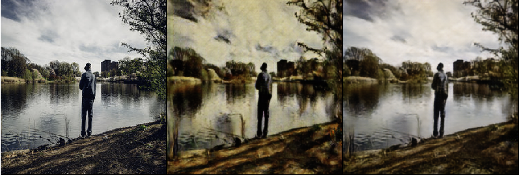
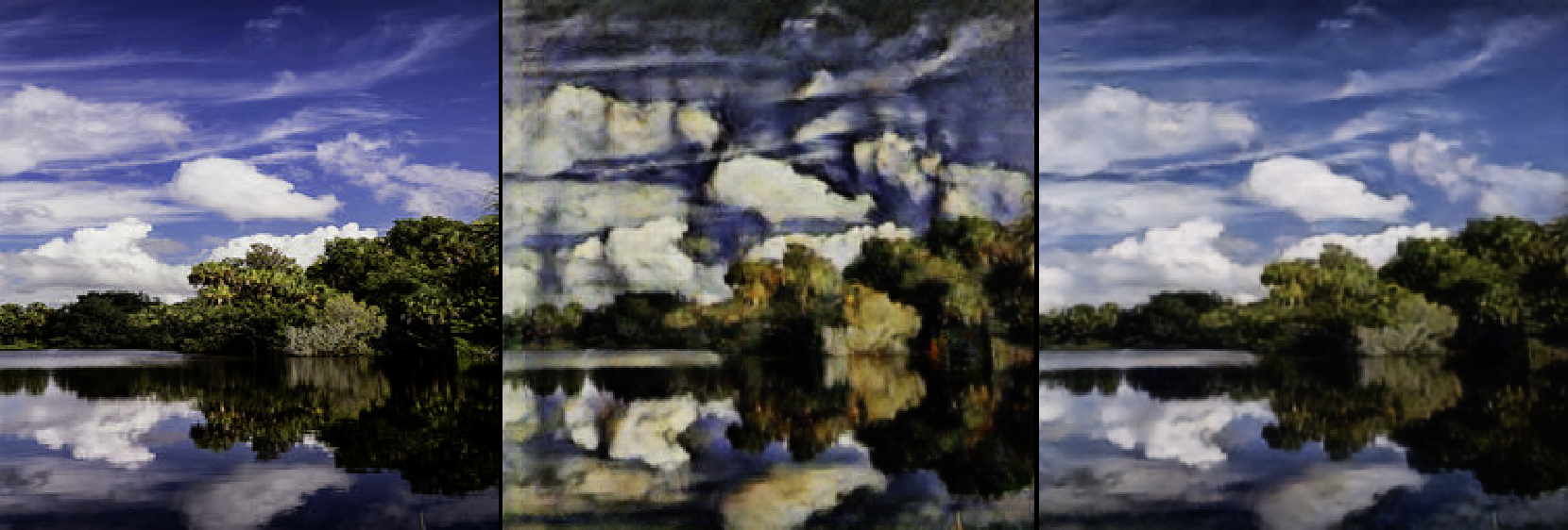
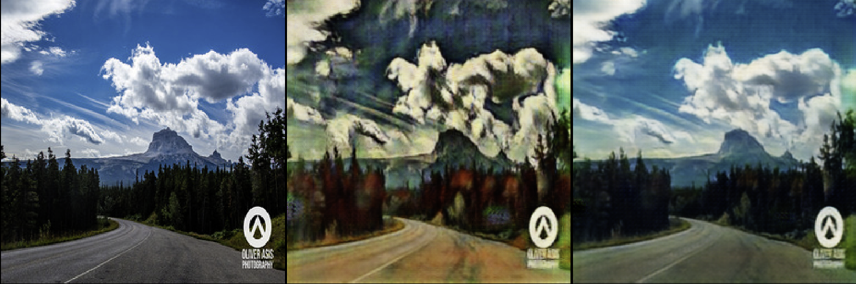
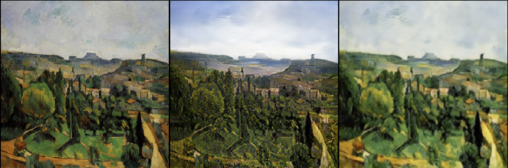
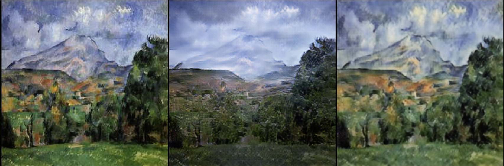
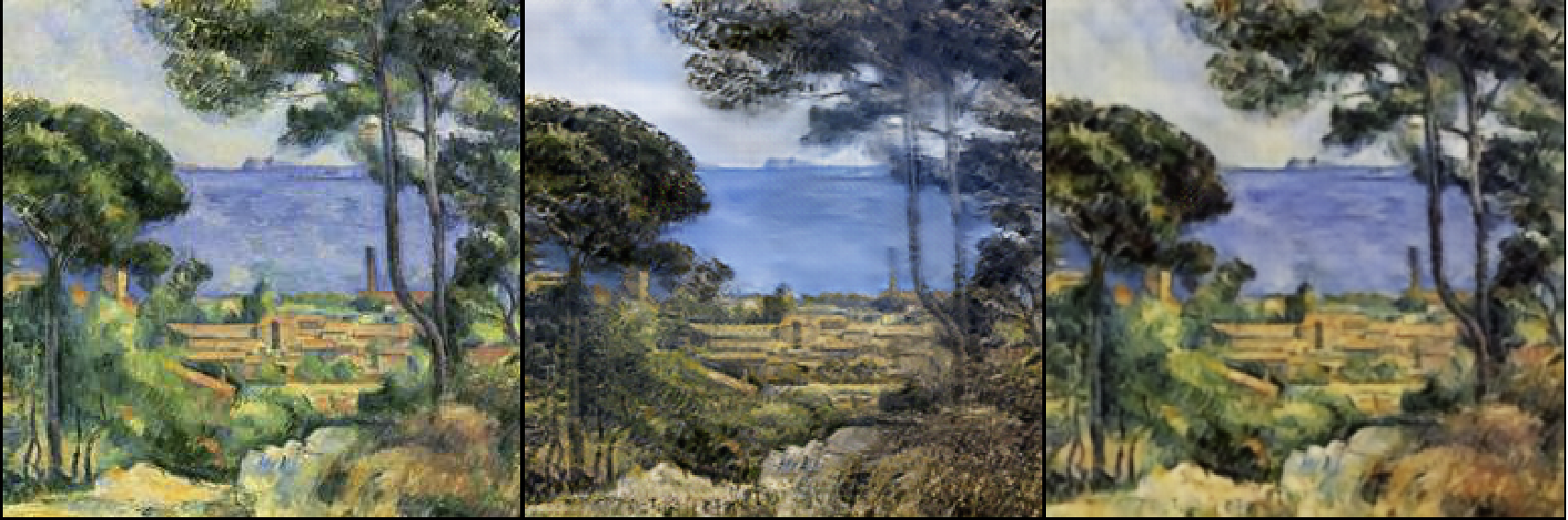
For painting → photo, the authors found that it was helpful to introduce an additional loss to encourage the mapping to preserve color composition between the input and output. In particular, they regularized the generator to be near an identity mapping when real samples of the target domain are provided as the input to the generator:

$$\mathcal{L}_{\text{identity}}(G, F) = \mathbb{E}_{y \sim p_{\text{data}}(y)} \left[ | G(y) - y |_1 \right] + \mathbb{E}_{x \sim p_{\text{data}}(x)} \left[ | F(x) - x |_1 \right]$$

Key Takeaways

• It is difficult to optimize the adversarial objective in isolation — standard procedures often lead to the well-known problem of mode collapse. Both the mappings $G$ and $F$ are trained simultaneously to enforce the structural assumption.
• The translation should be Cycle consistent; mathematically, translator $G: X \to Y$ and another translator $F: Y \to X$ should be inverses of each other (and both mappings should be bijections).
• It is similar to training two autoencoders — $F \circ G: X \to X$ jointly with $G \circ F: Y \to Y$. These autoencoders have a special internal structure — map an image to itself via an intermediate representation that is a translation of the image into another domain.
• It can also be treated as a special case of adversarial autoencoders, which use an adversarial loss to train the bottleneck layer of an autoencoder to match an arbitrary target distribution.

Network Architecture

Generator

Authors adopted the Generator's architecture from the neural style transfer and super-resolution papers. The network contains two stride-2 convolutions, several residual blocks, and two fractionally-strided convolutions with stride 1/2. 6 or 9 ResBlocks are used in the generator depending on the size of the training images. Instance normalization is used instead of batch normalization.

• 128 × 128 images: c7s1-64, d128, d256, R256, R256, R256, R256, R256, R256, u128, u64, c7s1-3
• 256 × 256 images: c7s1-64, d128, d256, R256, R256, R256, R256, R256, R256, R256, R256, R256, u128, u64, c7s1-3

Discriminator

The same 70 × 70 PatchGAN discriminator is used, which aims to classify whether 70 × 70 overlapping image patches are real or fake (more parameter efficient compared to a full-image discriminator). To reduce model oscillations, discriminators are updated using a history of generated images rather than the latest ones with a probability of 0.5.

• 70 × 70 PatchGAN: C64 - C128 - C256 - C512

Notation key

• c7s1-k — 7 × 7 Convolution + InstanceNorm + ReLU, k filters, stride 1.
• dk — 3 × 3 Convolution + InstanceNorm + ReLU, k filters, stride 2.
• Rk — residual block with two 3 × 3 convolutional layers, same number of filters on both.
• uk — 3 × 3 Deconv + InstanceNorm + ReLU, k filters, stride 1/2.
• Ck — 4 × 4 Convolution + InstanceNorm + LeakyReLU, k filters, stride 2.

Reflection padding is used to reduce artifacts. After the last layer, a convolution is applied to produce a 3-channel output for the generator and a 1-channel output for the discriminator. No InstanceNorm is applied in the first C64 layer.

Results

Photo → Cezanne Paintings

Cezanne Paintings → Photo

Where it went from here

CycleGAN demonstrated unpaired translation between two domains, with deterministic outputs and one network per direction. Two follow-ups pushed in interesting directions: generalizing to many domains with a single model, and questioning whether the cycle consistency assumption was even necessary in the first place.

No code or results for either of these in this post — the writeups below are just for reference.

StarGAN — Unified Generative Adversarial Networks for Multi-Domain Image-to-Image Translation — Choi et al. (2018)

If you want to translate between $N$ domains using CycleGAN, you have to train $N \times (N-1)$ generators (one per direction per pair) and a comparable number of discriminators. StarGAN replaces this with a single generator $G(x, c)$ that takes the input image $x$ and a target-domain label $c$, and a single discriminator $D$ with two heads: one that judges real-vs-fake as in any GAN, and one that classifies which domain the image belongs to ($D_{\text{cls}}$).

The training objective combines three loss terms:

• Adversarial loss for the real/fake head of $D$.
• Domain classification loss — on real images for $D$ (learns to classify domain correctly), and on fake images for $G$ (encourages $G$ to produce images that get classified into the target domain $c$).
• Reconstruction loss, in the same spirit as CycleGAN's cycle consistency: $G(G(x, c'), c)$ should reconstruct $x$. With a single generator, "cycle" is now $G$ applied twice with different target labels.

The headline applications were facial attribute editing on CelebA (hair color, gender, age) and expression transfer on RaFD. StarGAN also introduced a "mask vector" trick that lets you train on multiple datasets with non-overlapping attribute sets — useful when no single dataset has all the labels you care about.

The conceptual upgrade over CycleGAN is that domain identity becomes a conditioning input rather than something baked into the network's weights. One model, many directions, with a fixed parameter budget.

CUT — Contrastive Learning for Unpaired Image-to-Image Translation — Park et al. (2020)

This one is interesting because it questions the load-bearing assumption of CycleGAN. Cycle consistency requires training two generators ($G: X \to Y$ and $F: Y \to X$) and two discriminators, with the constraint that $F(G(x)) \approx x$. CUT argues that this is overkill — you can get the "preserve content from the input" effect with a much lighter mechanism, and only need one generator and one discriminator.

The replacement is a patchwise contrastive loss (PatchNCE). The intuition: a patch at location $(i, j)$ in the input $x$ should correspond to the patch at the same location $(i, j)$ in the output $G(x)$. If you extract features at that location from both, they should be close to each other (positive pair). They should be far from features at other locations in the same input image (negative pairs).

Concretely, feature embeddings are taken from multiple layers of the encoder half of the generator $G$ (which doubles as a feature extractor). For each spatial query location in $G(x)$, the InfoNCE loss is computed against features at other locations in $x$ as negatives. The loss is summed across multiple encoder layers, so matching happens at multiple scales.

The result: one generator, one discriminator, only the $X \to Y$ direction trained — with quality comparable to or better than CycleGAN on standard benchmarks (horse↔zebra, cat↔dog, photo↔painting). Training is faster and uses less memory, and the contrastive framing connects cleanly to the broader self-supervised learning literature that was taking off around the same time. The authors (much of the same team as CycleGAN) effectively frame this as: do you actually need a cycle? — and the answer turns out to be no, you just need a way to encourage the output to preserve content from the input, which contrastive matching does directly.

---

Closing thoughts

That's the arc of this post: NST shows that you don't need to train anything at all — pick a pretrained classifier, set up the right loss, and optimize a single image directly. Pix2Pix shows that with paired data, a conditional GAN can learn a whole class of translation tasks with one recipe. CycleGAN shows that even paired data isn't strictly required — cycle consistency is enough to learn a coherent mapping between two unpaired sets of images.

Generative image models have come a long way since these papers landed. If you'd like to keep going, the natural next steps are StyleGAN (for unconditional high-resolution generation), and more recently diffusion models (which have largely replaced GANs at the frontier of image generation). But the ideas in these three papers — perceptual losses, conditional generation, cycle consistency — keep showing up in different forms across all of them.

---

Updates

2020/11/20

Support of PyTorch Lightning added to Neural Style Transfer, CycleGAN, and Pix2Pix. Thanks to @William!

Why PyTorch Lightning?

• Easy to reproduce results
• Mixed Precision (16 bit and 32 bit) training support
• More readable by decoupling the research code from the engineering
• Less error prone by automating most of the training loop and tricky engineering
• Scalable to any hardware without changing the model (CPU, Single/Multi GPU, TPU)